Counting Without Loops: Difference Arrays and Cumulative Sums in R
Track 03 · Performance & Optimization · Tutorial
R
Performance
Microsimulation
Algorithms
Tutorial
Age-based counting functions in a microsimulation are easy to write as nested loops and brutally slow at scale. This tutorial rebuilds them with a difference-array and cumulative-sum kernel — turning every range update into two events and one cumsum() — and benchmarks the speedup live in R.
Author
Roa, J.
Published
May 22, 2026
Counting Without Loops
May 2026
Roa, J.
Laurent de La Hyre — Allegory of Arithmetic (c. 1650)Walters Art Museum · Baltimore La Hyre’s personification of Arithmetic turns from her ledger to display the tablet of Pythagoras — the integers 1 through 12, the even and the odd. The totals beneath her finger are reached the only way arithmetic allows: one carry at a time, each line the running sum of the last. The whole tutorial is hiding in that gesture.
A microsimulation simulates individual life histories and summarises them — how many people are alive at each age, how many carry a lesion, and at what sizes. Computing the summary once is cheap. Calibration recomputes it for every candidate parameter set, thousands of times over, so the counting functions that produce it have to be fast.
This tutorial rebuilds one of them. I started from how the counts were already being computed — a nested loop that dominated the calibration runtime — and, after some research, arrived at the difference array, recovered with R’s cumsum(). We build the counter from scratch on a small synthetic dataset and benchmark it.
The counting problem
Each simulated person is alive and at risk over a half-open age interval [start, stop) — present at age start, gone by age stop. We want a single vector: how many people are alive at each age on a fixed grid.
Show / hide code
simulate.R
simulate_people<-function(n, max_age=100L, seed=42L){set.seed(seed)start<-sample.int(max_age-1L, n, replace =TRUE)# entry age, 1..max_age-1span<-1L+rgeom(n, prob =1/18)# years at risk (mean ~18)stop<-pmin(start+span, max_age)# exit age, capped, half-opendata.frame(start =start, stop =stop)}v_ages<-1:100# the age grid we report onpeople<-simulate_people(2e4)# 20,000 life historieshead(people, 4)
  start stop
1    49   60
2    65  100
3    25   26
4    74   83
NoteOne convention, stated once
The at-risk window is half-open: a person counts at every age a with start ≤ a < stop. Fix the convention once and apply it everywhere — most off-by-one bugs in this code come from a convention that drifted.
The obvious way (and why it hurts)
The direct approach: for each person, increment a counter at every age they are alive. Two nested loops:
This is correct but slow. The inner loop runs once per person-year: with N people each alive for about A ages, the cost is O(N × A). Both factors grow with the model, and the whole computation repeats on every calibration step. This was the bottleneck.
The trick: turn a range into two events
The key observation: a count over the range [start, stop) only changes at the two ends. Every age in between holds the same value, so filling them in one at a time is wasted work.
Record only the two points where the count changes:
at age start, the running count goes up by 1,
at age stop, it goes down by 1.
Store those +1/−1 events in a difference arrayd. The count at every age is then the cumulative sum of d. A range update becomes two point updates plus one pass.
NoteWhere this comes from
This is a classic data structures & algorithms technique — the difference array paired with a prefix sum (the cumsum). Adding a constant across a whole range [l, r) becomes two point updates (+1 at l, −1 at r), and the running prefix sum rebuilds the value everywhere. Counting how many intervals overlap each point this way is the sweep-line / event-counting pattern, known in competitive programming as the imos method.
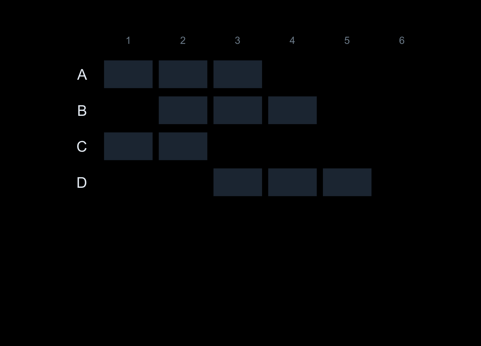
Worked by hand on four people:
Person
start
stop
alive at ages
A
1
4
1, 2, 3
B
2
5
2, 3, 4
C
1
3
1, 2
D
3
6
3, 4, 5
Show / hide code
worked-example.R
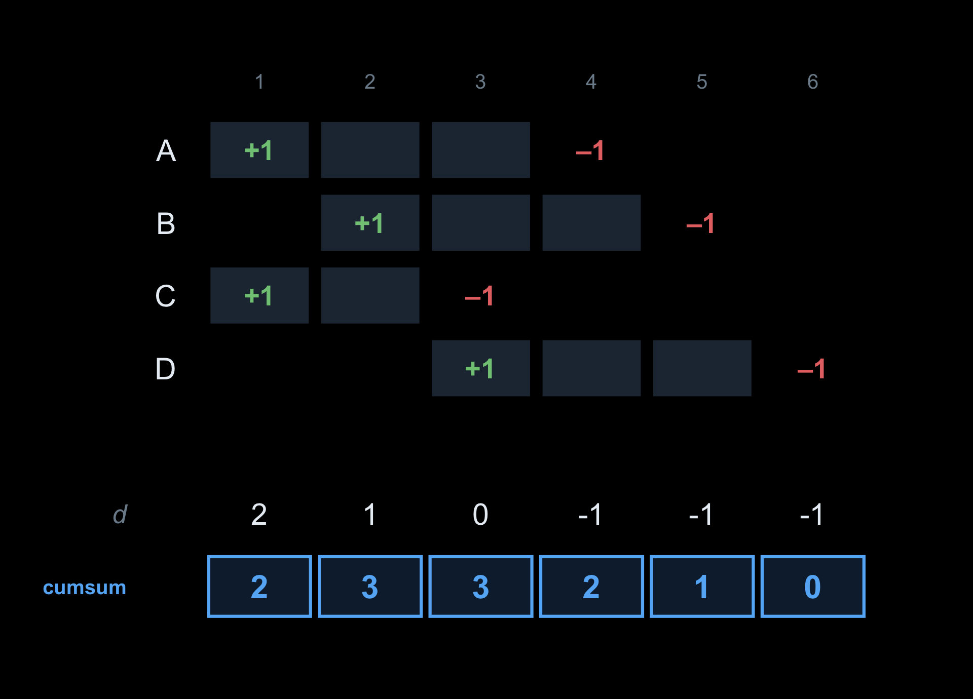
demo<-data.frame(start =c(1L, 2L, 1L, 3L), stop =c(4L, 5L, 3L, 6L))starts<-tabulate(demo$start, nbins =6)# +1 where intervals beginstops<--tabulate(demo$stop, nbins =6)# -1 where intervals endd<-starts+stopsrbind(`+1 at start` =starts, `-1 at stop` =stops, `delta d` =d, `alive = cumsum(d)` =cumsum(d))
The last row — 2 3 3 2 1 0 — is the answer, and you can check it by eye against the table. We never touched the insides of any interval. tabulate() did the bookkeeping (it counts how many values fall in each integer bin), and cumsum() did the sweep.
The idea, in motion
Scroll the table to the right and watch the count build itself — two marks per person, then one sweep.
Four people, six overlapping years. The question every summary asks: how many are alive at each age?
The slow way counts every cell. The fast way touches only the edges — two marks per person, then one sweep.
Four people, four overlapping spans. Each faint cell is one person-year — what the nested loop visits, one at a time.
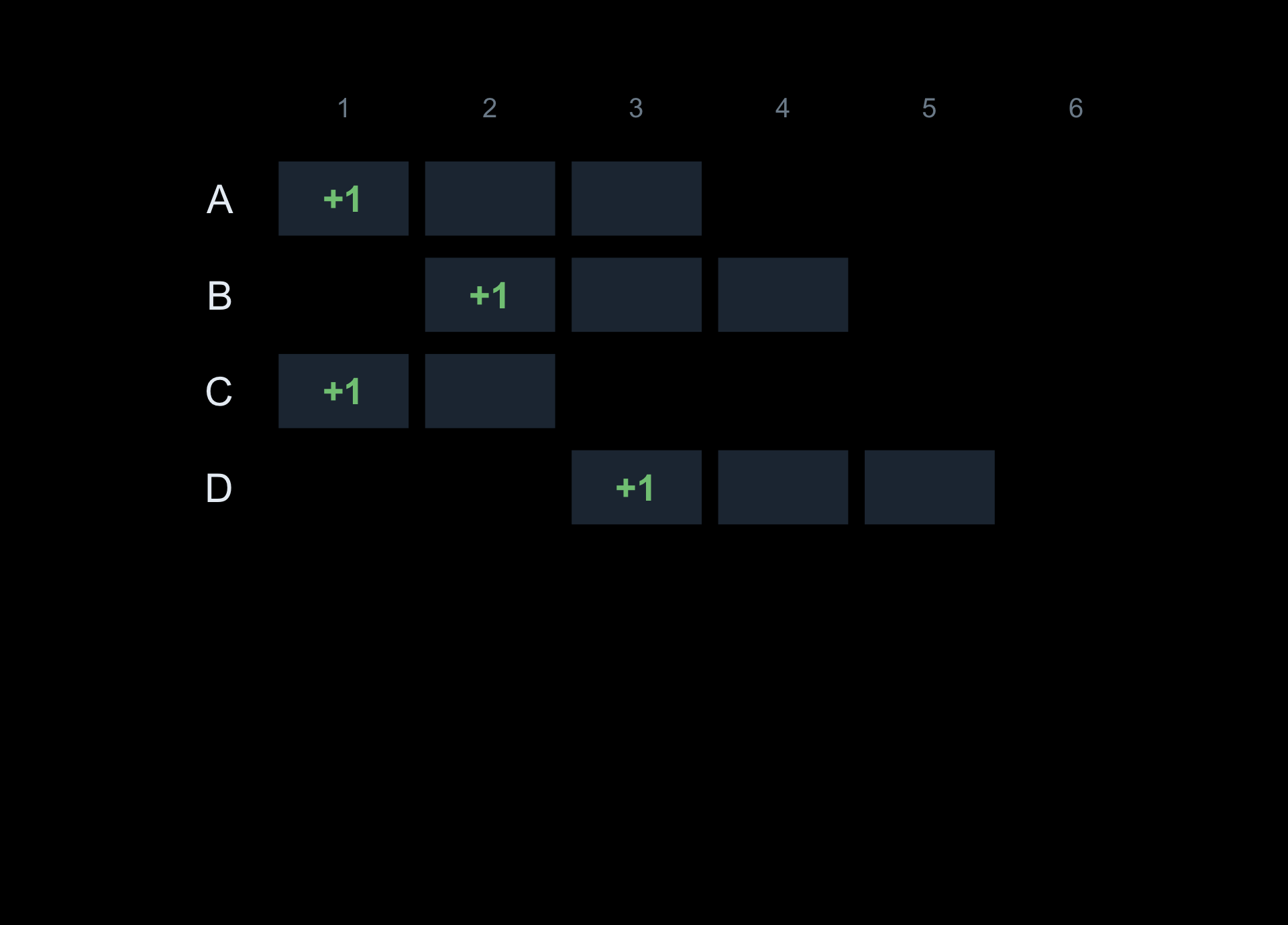
The count only moves at the edges of a span. At each start, add +1.
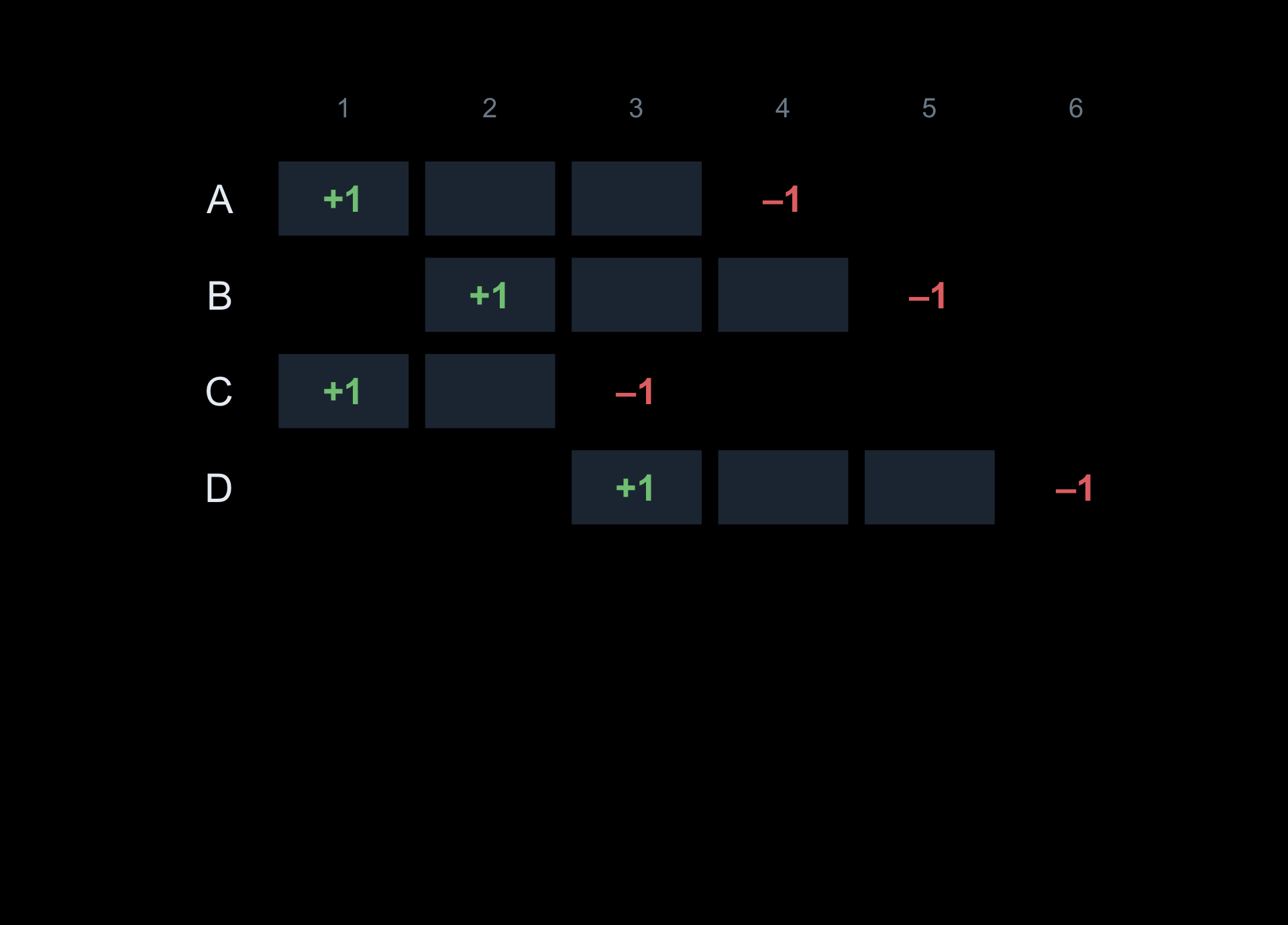
At each stop, subtract 1. Two marks per person — never the middle.
Zoom in on the first person: +1 at the start, −1 at the stop, nothing in between.
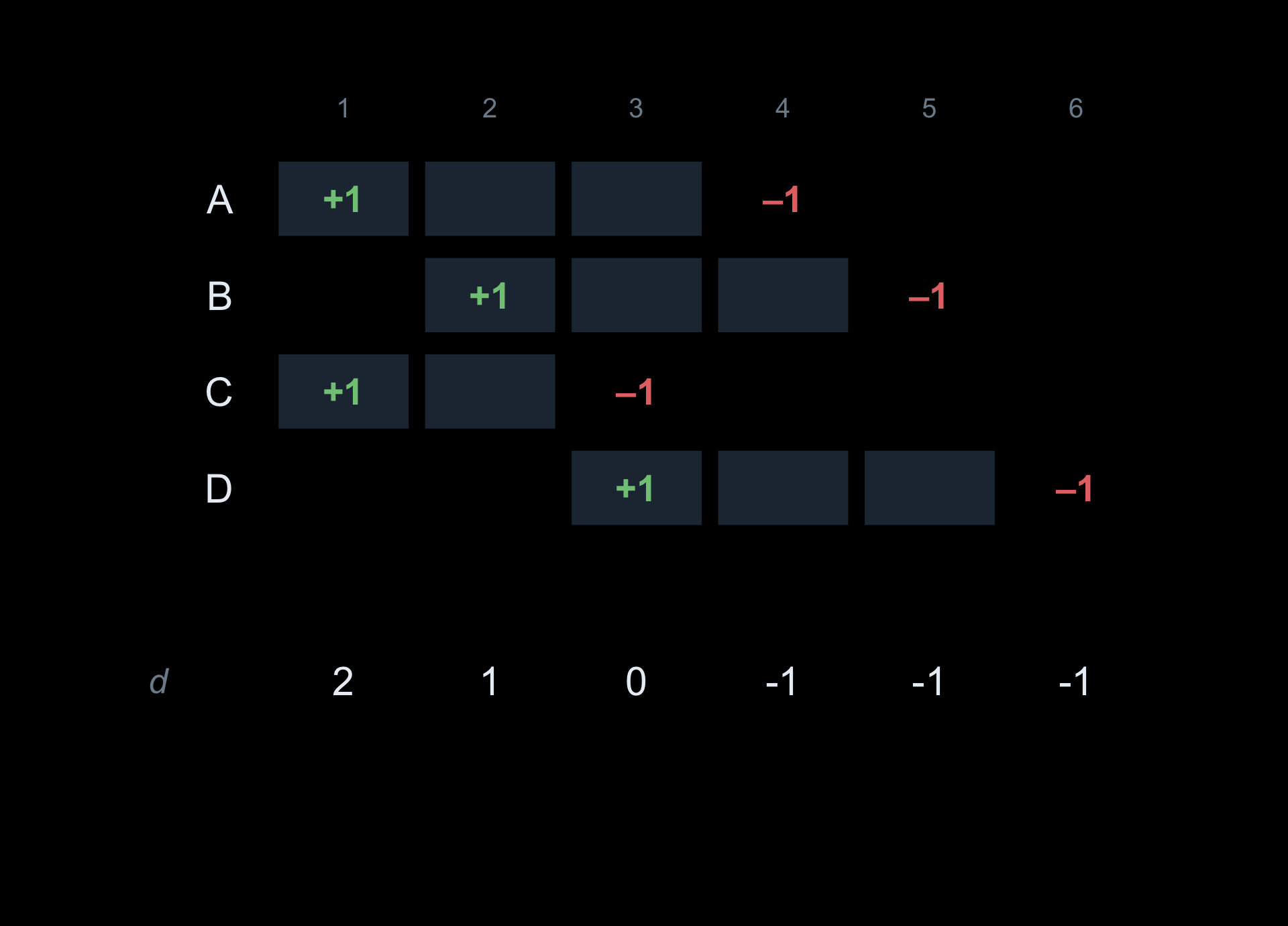
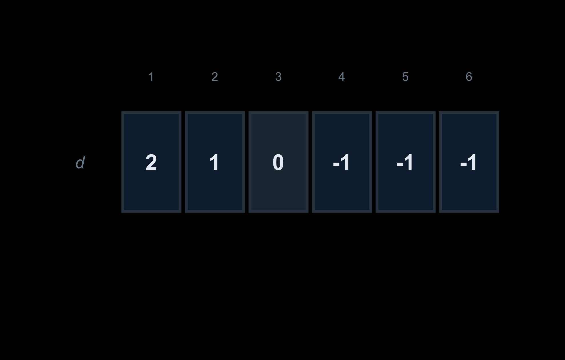
Add the columns: that is the difference array, d.
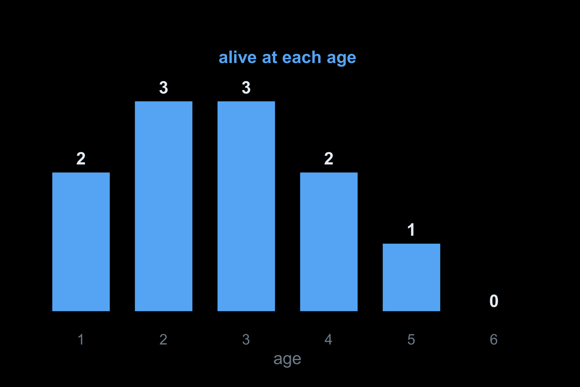
Sweep left to right with cumsum(d). The running total is the number alive at every age: 2 3 3 2 1 0.
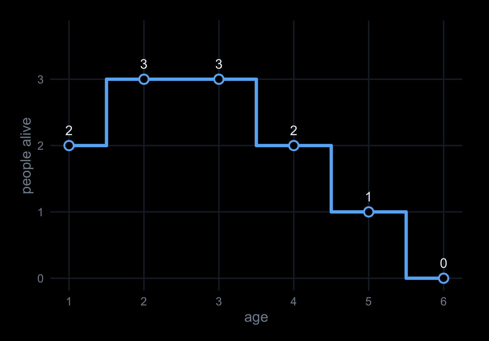
Plot the running total against age: a survival curve, the model’s actual output — from two marks and one sweep.
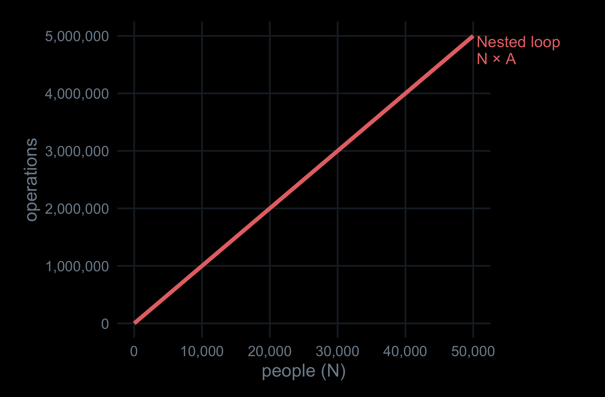
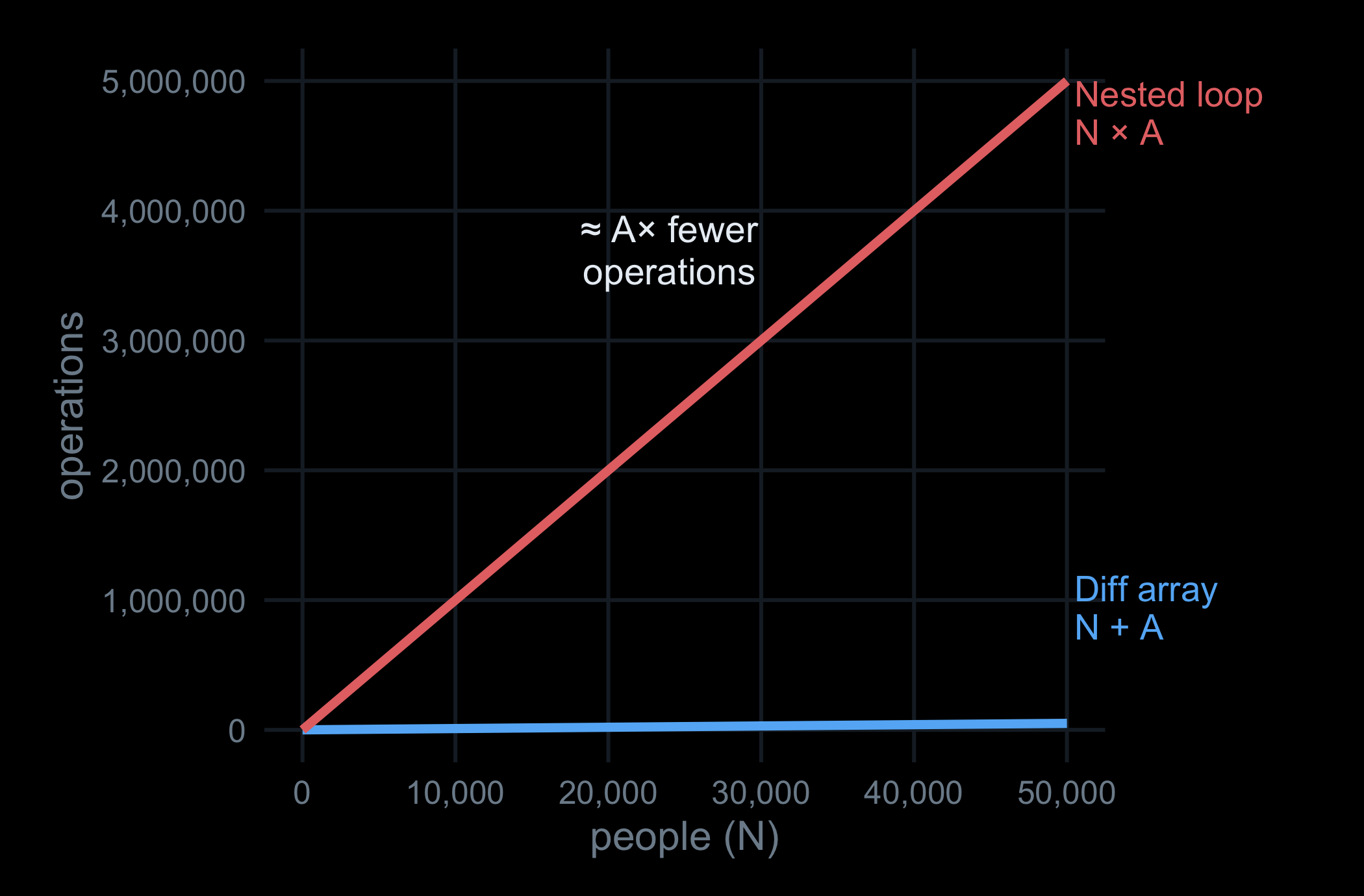
Now scale it up. The nested loop does one operation per person-year — N × A of them. A hundred ages and tens of thousands of people, and that climbs fast.
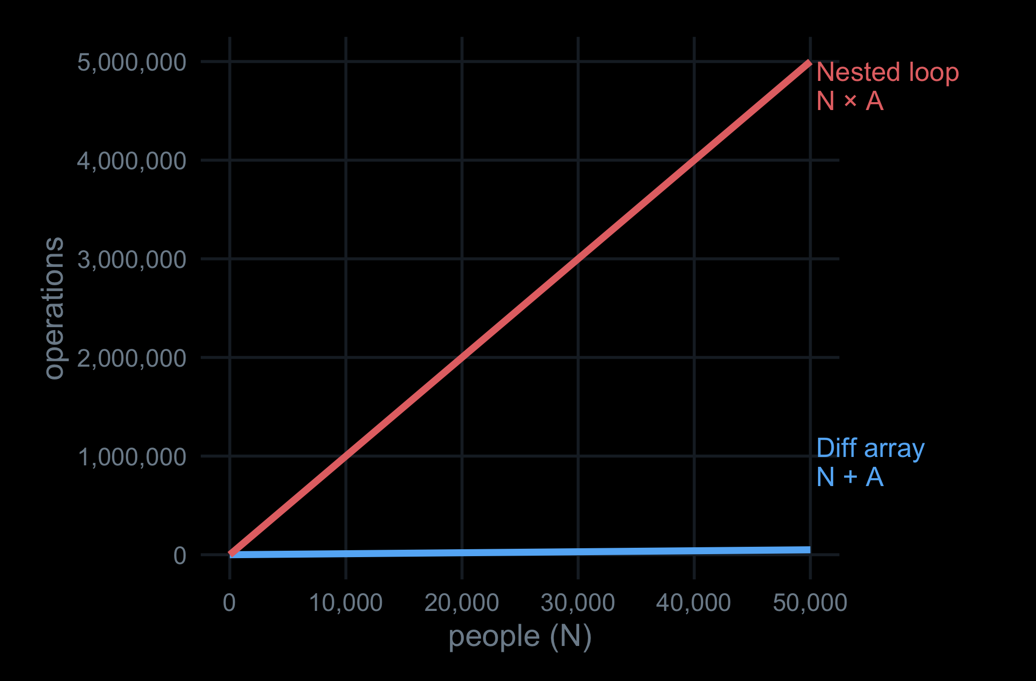
The difference array does one operation per person, plus one sweep of the ages — N + A. On the same axes it barely leaves the floor.
That gap is the whole story: the same answer for a fraction of the work, and it only widens with every extra life you simulate.
The vectorised version
This collapses into a function with no R-level loop:
Show / hide code
fast-count.R
count_alive_diff<-function(start, stop, v_ages){n<-length(v_ages)# +1 where intervals begin, -1 where they end (half-open [start, stop))d<-tabulate(start, nbins =n)-tabulate(stop, nbins =n)cumsum(d)}identical(count_alive_naive(people$start, people$stop, v_ages),count_alive_diff(people$start, people$stop, v_ages))
[1] TRUE
Same result, O(N + A): one pass to place the events, one pass for the cumulative sum.
TipPass the grid in, don’t rebuild it
v_ages is an argument, not a constant inside the function. The age grid is identical across calibration iterations, so rebuilding it inside each call wastes work. As a parameter, the same kernel serves any age range and the hot path avoids redundant allocation.
Many categories at once: change points
The same kernel handles every stratified count in the summary. If each lesion is active over its own [onset, regress) window, count active lesions by age by building the difference array over the lesion events instead of the person events:
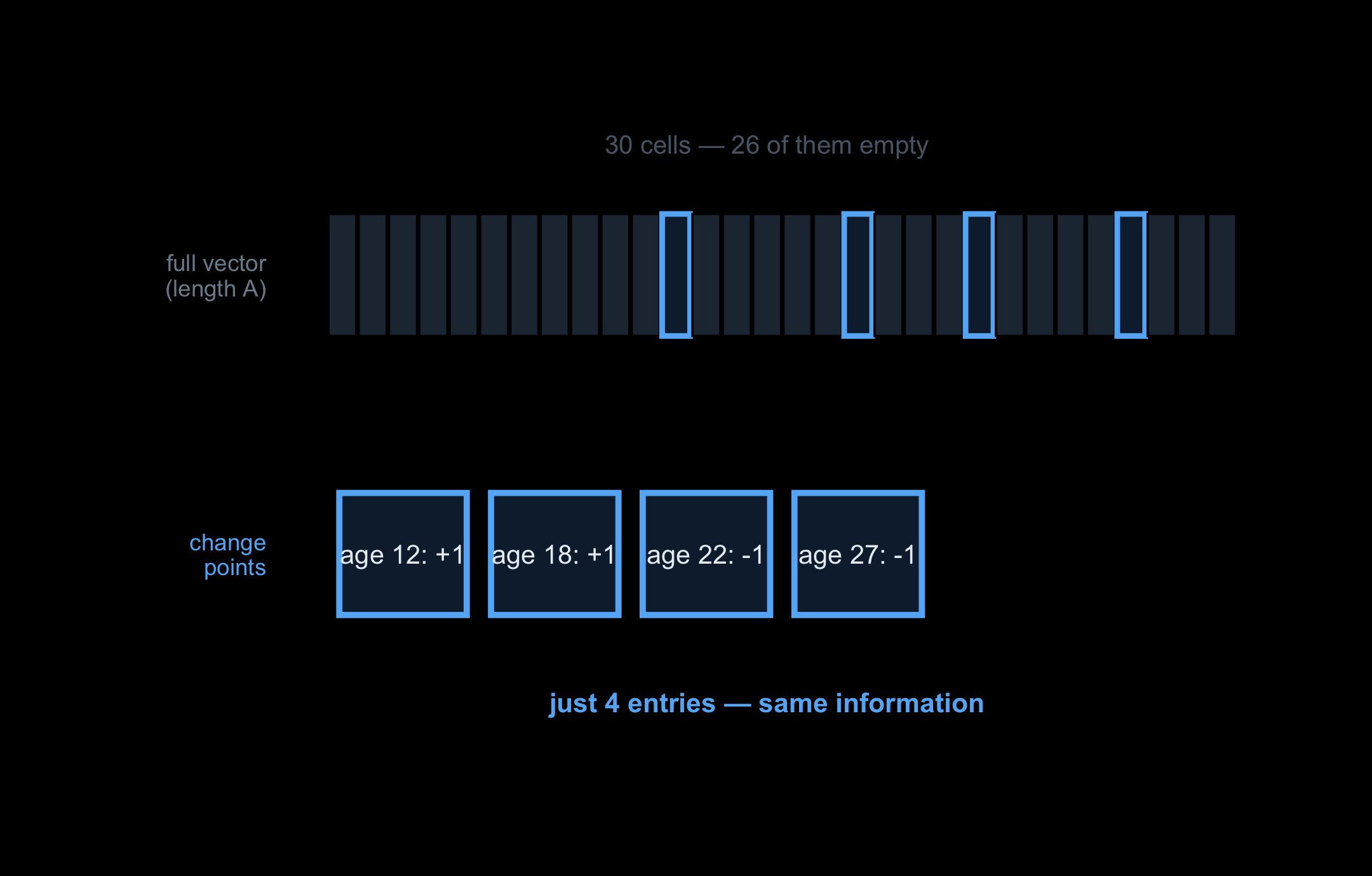
The difference array d is itself the change-point representation: its non-zero entries are the only ages where the count moves. For a sparse category — a lesion size present at only a few ages — there is no need to materialise a length-A vector. Store the (age, delta) pairs at the change points and sum them on demand; a stratified summary becomes a short list of events per category.
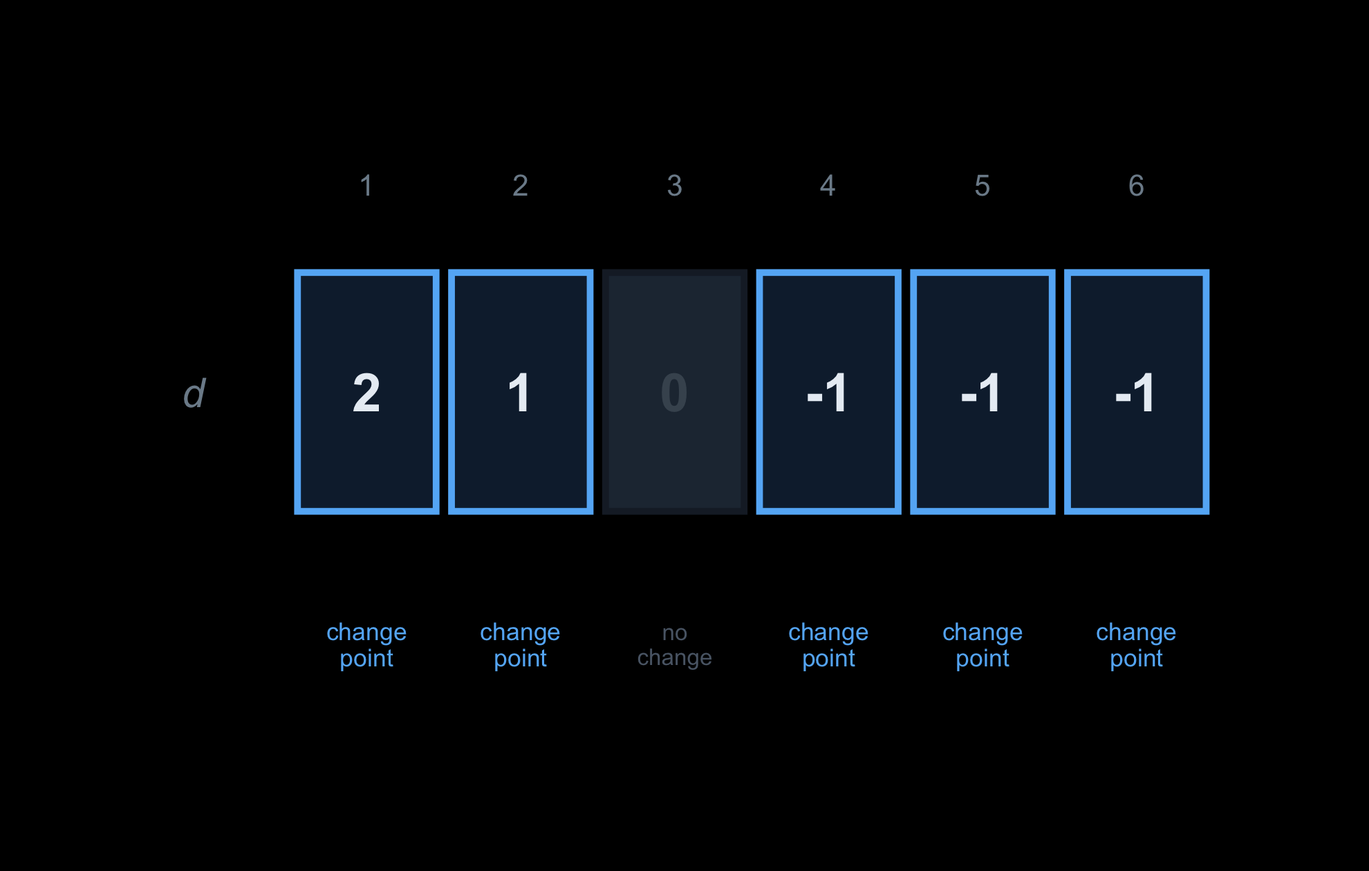
The same difference array again: 2 1 0 −1 −1 −1.
Only the non-zero entries matter — the change points, the ages where the count moves. At age 3 it does not change.
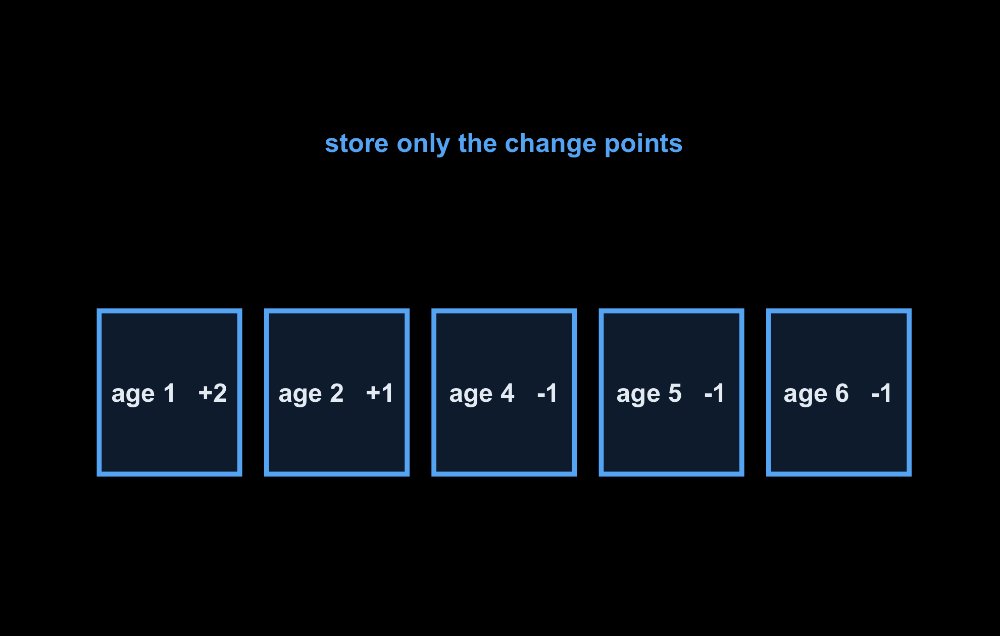
So drop the rest of the row. Keep only the (age, delta) pairs at the change points; everything between them is implied.
For a sparse category — active at only a few ages — the full length-A vector is mostly empty, but its change points are a tiny list. That list is the compressed summary.
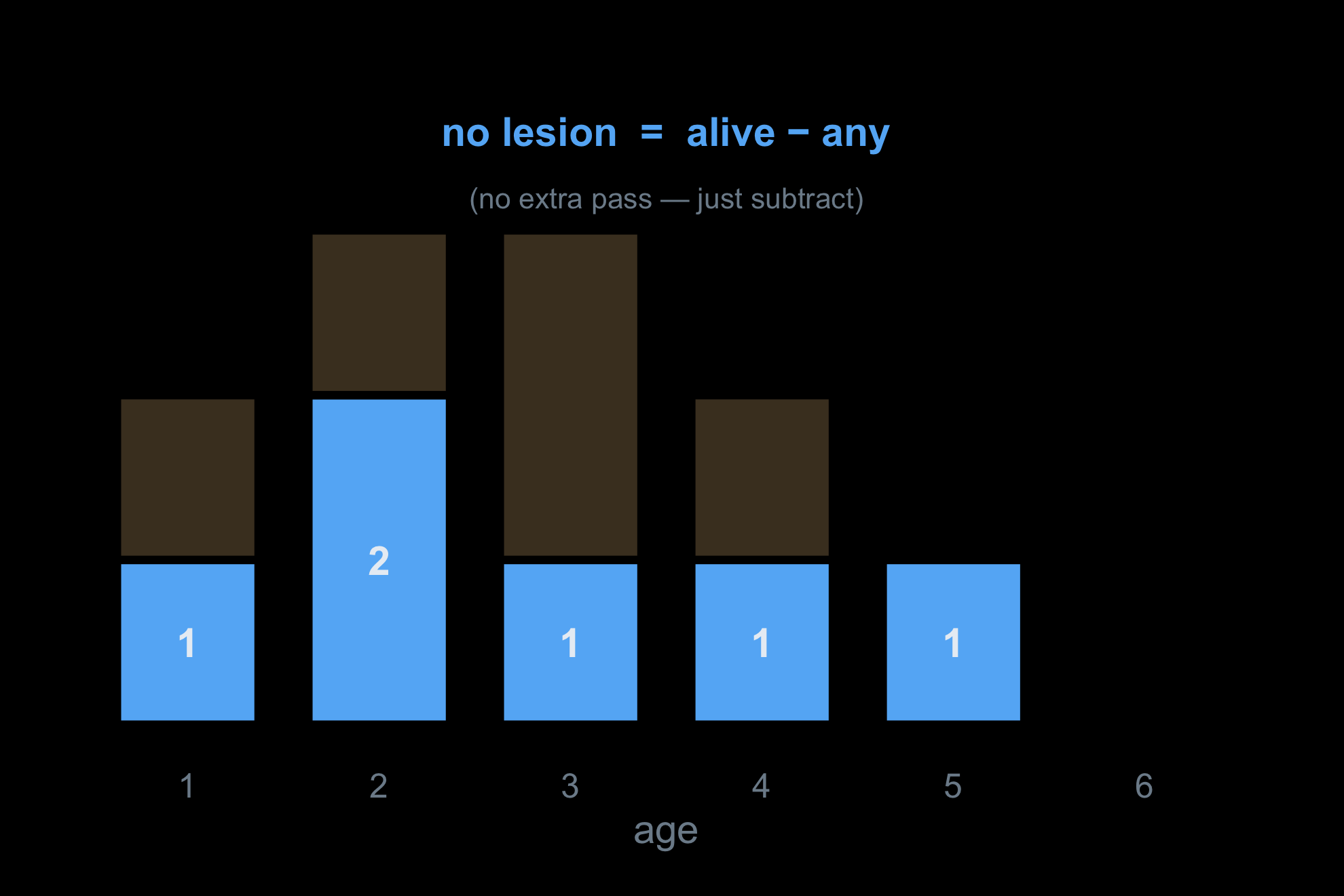
Counting the complement: alive − any
The count of people with zero lesions at each age does not need a third pass. It is a subtraction:
Show / hide code
complement.R
# alive-by-age (from before) and the count of people with >= 1 active lesion,# built from each PERSON's "any lesion active" window (one row per person, not per lesion)alive<-count_alive_diff(people$start, people$stop, v_ages)# (illustrative) suppose any_start / any_stop bound each person's lesion-bearing span:any_start<-people$start+5Lany_stop<-pmin(people$stop, people$start+15L)n_any<-count_alive_diff(any_start, any_stop, v_ages)n_zero<-alive-n_any# people with no active lesion, by agehead(n_zero, 8)
[1] 204 421 613 816 1033 1036 1005 1012
At each age every person either has a lesion or does not, so zero = alive − any. One subtraction replaces an extra sweep. Build n_any from each person’s lesion-bearing window, counted once — not per lesion — or a person with three lesions is subtracted three times.
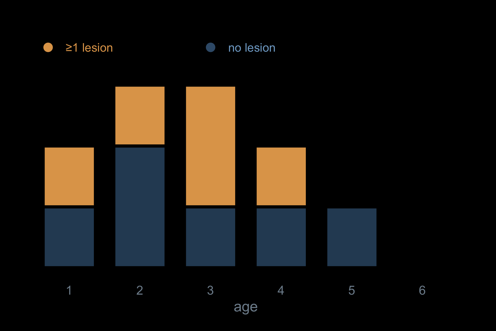
Start with everyone alive at each age — the count already built.
Some of them carry a lesion. Split each bar: the amber part is everyone with ≥1 lesion.
The blue part is everyone with no lesion — exactly alive − any. No third pass; one subtraction.
Does it actually pay off?
Measured directly, same population and grid, the two functions head to head:
Show / hide code
benchmark.R
library(microbenchmark)mb<-microbenchmark("Nested loop"=count_alive_naive(people$start, people$stop, v_ages),"Diff array + cumsum"=count_alive_diff(people$start, people$stop, v_ages), times =10)print(mb, unit ="ms")
Unit: milliseconds
                expr       min        lq      mean     median        uq
         Nested loop 19.822680 20.002055 20.230704 20.0864945 20.151705
 Diff array + cumsum  0.027634  0.028536  0.040139  0.0324105  0.054243
       max neval cld
 21.696462    10  a
  0.059696    10   b
At 20,000 people the difference-array version is about 620× faster than the nested loop, and the gap widens with N because the two functions are on different complexity curves:
Figure 1: Median time per call vs. population size, log–log. The nested loop (O(N × A)) climbs with the population; the difference-array kernel (O(N + A)) stays nearly flat across three orders of magnitude.
On the log–log axes the nested loop rises at a constant slope (polynomial growth); the difference-array kernel stays nearly flat — at a million people it does essentially the same two passes it did at a thousand.
The same numbers, sortable:
Takeaways
The key points:
A range update is two events. Whenever you find yourself incrementing a counter across an interval, record +1 at the start and −1 at the end instead, then cumsum(). Loop over boundaries, never over insides.
tabulate() + cumsum() is the R idiom.tabulate() bins the events without a loop; cumsum() sweeps them into running totals. Together they replace the double loop with O(N + A) arithmetic.
The difference array is also the change-point store. Its non-zero entries are the only ages where the count moves — keep just those for sparse, stratified categories.
Complements are subtractions.zero = alive − any. Don’t re-sweep for the inverse of something you already counted.
Hoist the invariants. Passing the age grid in as v_ages keeps it from being rebuilt on every one of thousands of calibration calls.
ImportantWhy this was worth a tutorial
The model behind this was a colorectal-cancer microsimulation; its summary functions ran on every calibration iteration, thousands of times per fit. Rewriting them around the difference-array + cumsum kernel, and passing the age grid as a v_ages argument instead of rebuilding it each call, cut end-to-end calibration time by roughly 60%. The counting kernel alone improved by far more, as the benchmark shows; calibration carries other costs. Same results, a fraction of the runtime.