Bias in AI: Detection and Mitigation

Track 02 · Fairness in ML · Tutorial

A hands-on COMPAS case study using Aequitas for group-level fairness metrics and AIF360 for reweighing-based bias mitigation. Covers demographic exploration, false-positive disparity by race, and pre-/post-processing mitigation with native Python chunks.

Bias in AI: Detection and Mitigation

December 2022 · Berlin

Roa, J., Greß, C., Schweren, H.

Raphael — The School of Athens (1509–1511) Stanza della Segnatura, Apostolic Palace · Vatican City Plato and Aristotle walk side by side at the vanishing point of a vast barrel-vaulted basilica, encircled by fifty philosophers, geometers, and astronomers of antiquity. Raphael controls the crowd into a single breathing whole — each cluster drawing the eye inward to the center. Art historians call it the definitive image of High Renaissance clarity and equilibrium.

  Objective

A walk-through of how to detect algorithmic bias in a real-world classifier and how to mitigate it without rebuilding the model from scratch. The teaching corpus is the COMPAS Recidivism Risk Score Dataset released by ProPublica in 2016 — the canonical case study for fairness research because the bias is well-documented, the labels are real, and the impact (sentencing decisions) is concrete. Originally a Deep Learning assignment in the M.Sc. Data Science for Public Policy programme at the Hertie School, the materials were authored by Jorge Roa with co-authors Carlo Greß and Hannah Schweren.

  The COMPAS dataset

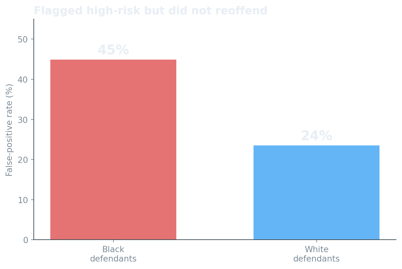
COMPAS (Correctional Offender Management Profiling for Alternative Sanctions) is a commercial risk-assessment tool used by US courts to predict whether a defendant will reoffend within two years. In 2016 ProPublica showed that the model’s false positive and false negative rates differ sharply by race — Black defendants are nearly twice as likely to be incorrectly flagged as future criminals than white defendants, and white defendants are more often incorrectly flagged as low-risk. The dataset they released has become the canonical fairness teaching corpus.

The two questions every fairness analysis tries to answer. (1) Is the model’s error rate equal across groups? If you’re more likely to be falsely flagged as high-risk because of your race, the answer is no. (2) Can we mitigate that without retraining? Yes — there are pre-processing (modify the data), in-processing (modify the loss), and post-processing (modify the predictions) techniques. This tutorial covers two pre-processing techniques (Disparate Impact Repairing, Reweighing) and one post-processing one (Reject Option Classification).

The headline finding from ProPublica’s 2016 investigation is a single, stark gap.

A false positive is a defendant the model flags as high-risk who then does not reoffend — a label that can cost someone bail or a harsher sentence.

Black defendants were falsely flagged at nearly twice the rate of white defendants — 45% against 23%. Same model, same threshold, opposite error burden.

That gap — not the model’s overall accuracy — is what a fairness audit exists to surface. The rest of this tutorial measures it with aequitas and then mitigates it with aif360.

  Setup

The libraries below cover the full pipeline: data wrangling, plotting, fairness metrics (aequitas), and bias-mitigation algorithms (aif360). The original assignment also explored a TensorFlow neural-network classifier; that part is omitted here to keep the tutorial portable.

• pandas · numpy — data wrangling and numeric arrays
• matplotlib · seaborn — plots styled to match the page
• scikit-learn — logistic regression, scaling, and train/test split
• aequitas — group-level fairness metrics: FPR / FNR by demographic
• aif360 — IBM’s AI Fairness toolkit: reweighing, disparate-impact metrics

setup.py

import warnings
warnings.filterwarnings("ignore")

import numpy as np
import pandas as pd
import matplotlib.pyplot as plt
import seaborn as sns

# Match the page's dark + transparent + #64B5F6 visual language
plt.rcParams.update({
    "figure.facecolor":  "none",
    "axes.facecolor":    "none",
    "savefig.facecolor": "none",
    "savefig.transparent": True,
    "text.color":        "#cfd8dc",
    "axes.labelcolor":   "#eceff1",
    "axes.edgecolor":    "#37474f",
    "xtick.color":       "#cfd8dc",
    "ytick.color":       "#cfd8dc",
    "axes.titlecolor":   "#ffffff",
    "axes.titlelocation": "left",
    "axes.titlesize":    13,
    "axes.titleweight":  "bold",
    "axes.spines.top":   False,
    "axes.spines.right": False,
    "grid.color":        "#37474f",
    "grid.linestyle":    "--",
    "grid.alpha":        0.4,
    "figure.figsize":    (9, 5),
    "figure.dpi":        110,
})

PAL = ["#64B5F6", "#FF8A65", "#81C784", "#FFCA28", "#BA68C8",
       "#4DD0E1", "#F48FB1", "#FFB74D"]
sns.set_palette(PAL)

  Data — load and inspect

The COMPAS data ships in two flavours alongside this tutorial: an aequitas-formatted version with categorical race / sex / age labels (good for fairness diagnostics) and a preprocessed numeric version (good for ML models). Both come from the original assignment repo.

load-aequitas.py

df = pd.read_csv("data/compas_for_aequitas.csv")
print(f"Rows: {df.shape[0]:,}   Cols: {df.shape[1]}")
df.head(5)

Rows: 7,214   Cols: 6

	entity_id	score	label_value	race	sex	age_cat
0	1	0.0	0	Other	Male	Greater than 45
1	3	0.0	1	African-American	Male	25 - 45
2	4	0.0	1	African-American	Male	Less than 25
3	5	1.0	0	African-American	Male	Less than 25
4	6	0.0	0	Other	Male	25 - 45

The columns are minimal on purpose: an entity id, the score (the COMPAS prediction), the label (whether the person actually re-offended within two years), and three protected attributes — race, sex, age_cat.

  Demographic breakdown

The first thing any fairness analysis does is count. If a group is severely under-represented in the training data, no metric will save you. Here, the dataset’s racial composition skews heavily toward two groups:

demographics.py

fig, axes = plt.subplots(1, 3, figsize=(13, 4))

for ax, col, title in zip(
    axes,
    ["race", "sex", "age_cat"],
    ["Race", "Sex", "Age category"]
):
    counts = df[col].value_counts()
    ax.bar(counts.index, counts.values, color=PAL[:len(counts)])
    ax.set_title(f"Defendants by {title}")
    ax.tick_params(axis="x", rotation=20)
    ax.set_ylabel("Count" if col == "race" else None)

plt.tight_layout()
plt.show()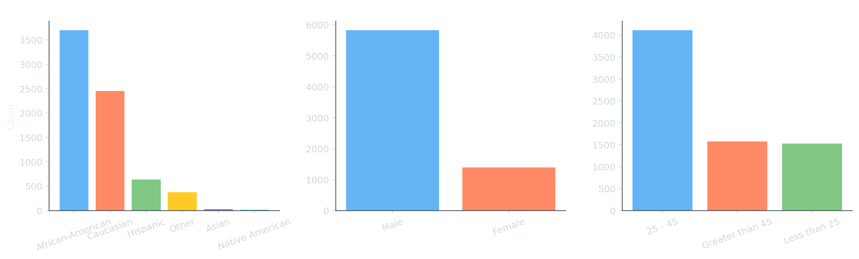

Two things stand out: African-American and Caucasian defendants together account for >90 % of the corpus, and men outnumber women by roughly four to one. Any bias the COMPAS model exhibits across race is therefore very visible across these two groups.

  Recidivism rates by demographic

label_value is the ground-truth two-year recidivism label. The base rates differ across groups, which is exactly the source of the COMPAS controversy — most fairness definitions are incompatible in a world where base rates differ.

recidivism-by-race.py

recid = (df.groupby("race")["label_value"]
           .agg(rate="mean", n="size")
           .sort_values("rate", ascending=False))
recid["rate"] = (recid["rate"] * 100).round(1)
recid

	rate	n
race
Native American	55.6	18
African-American	51.4	3696
Caucasian	39.4	2454
Hispanic	36.4	637
Other	35.3	377
Asian	28.1	32

recid-plot.py

fig, ax = plt.subplots(figsize=(8, 4))
recid_plot = recid.sort_values("rate")
ax.barh(recid_plot.index, recid_plot["rate"], color=PAL[0])
ax.set_xlabel("Two-year recidivism rate (%)")
ax.set_title("Observed recidivism rate by race")
for i, v in enumerate(recid_plot["rate"]):
    ax.text(v + 0.5, i, f"{v}%", va="center", color="#cfd8dc")
plt.tight_layout()
plt.show()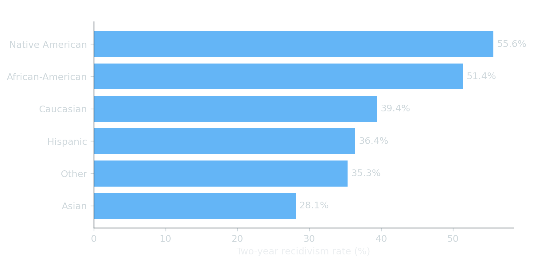

  Aequitas — group-level fairness metrics

Aequitas (built at the University of Chicago Data Science for Social Good lab) is a Python toolkit that turns a predictions + protected attributes dataframe into a fairness audit. Its core abstraction is groups — rows of the data partitioned by the values of a protected attribute — and its core operation is computing per-group metrics: false positive rate, false negative rate, true positive rate, and so on.

aequitas-group.py

from aequitas.group import Group

g = Group()
xtab, _ = g.get_crosstabs(df)

# The crosstab is wide — show the absolute-metrics columns only
abs_metrics = g.list_absolute_metrics(xtab)
xtab[["attribute_name", "attribute_value"] + abs_metrics].round(3)

	attribute_name	attribute_value	accuracy	tpr	tnr	for	fdr	fpr	fnr	npv	precision	ppr	pprev	prev
0	race	African-American	0.638	0.720	0.552	0.350	0.370	0.448	0.280	0.650	0.630	0.655	0.588	0.514
1	race	Asian	0.844	0.667	0.913	0.125	0.250	0.087	0.333	0.875	0.750	0.002	0.250	0.281
2	race	Caucasian	0.670	0.523	0.765	0.288	0.409	0.235	0.477	0.712	0.591	0.257	0.348	0.394
3	race	Hispanic	0.661	0.444	0.785	0.289	0.458	0.215	0.556	0.711	0.542	0.057	0.298	0.364
4	race	Native American	0.778	0.900	0.625	0.167	0.250	0.375	0.100	0.833	0.750	0.004	0.667	0.556
5	race	Other	0.666	0.323	0.852	0.302	0.456	0.148	0.677	0.698	0.544	0.024	0.210	0.353
6	sex	Female	0.654	0.608	0.679	0.243	0.487	0.321	0.392	0.757	0.513	0.178	0.424	0.357
7	sex	Male	0.654	0.629	0.676	0.330	0.365	0.324	0.371	0.670	0.635	0.822	0.468	0.473
8	age_cat	25 - 45	0.648	0.626	0.666	0.323	0.385	0.334	0.374	0.677	0.615	0.580	0.468	0.460
9	age_cat	Greater than 45	0.704	0.428	0.832	0.241	0.459	0.168	0.572	0.759	0.541	0.119	0.250	0.316
10	age_cat	Less than 25	0.617	0.740	0.459	0.425	0.360	0.541	0.260	0.575	0.640	0.301	0.653	0.565

Each row is one group (e.g. race=African-American, sex=Male, age_cat=25-45) with its full per-group confusion-matrix derivatives. fpr and fnr are the columns where the bias becomes visible.

  Plot the per-group false-positive rate

aequitas-fpr-plot.py

from aequitas.plotting import Plot
aqp = Plot()
fig = aqp.plot_group_metric(xtab, "fpr")
plt.tight_layout()
plt.show()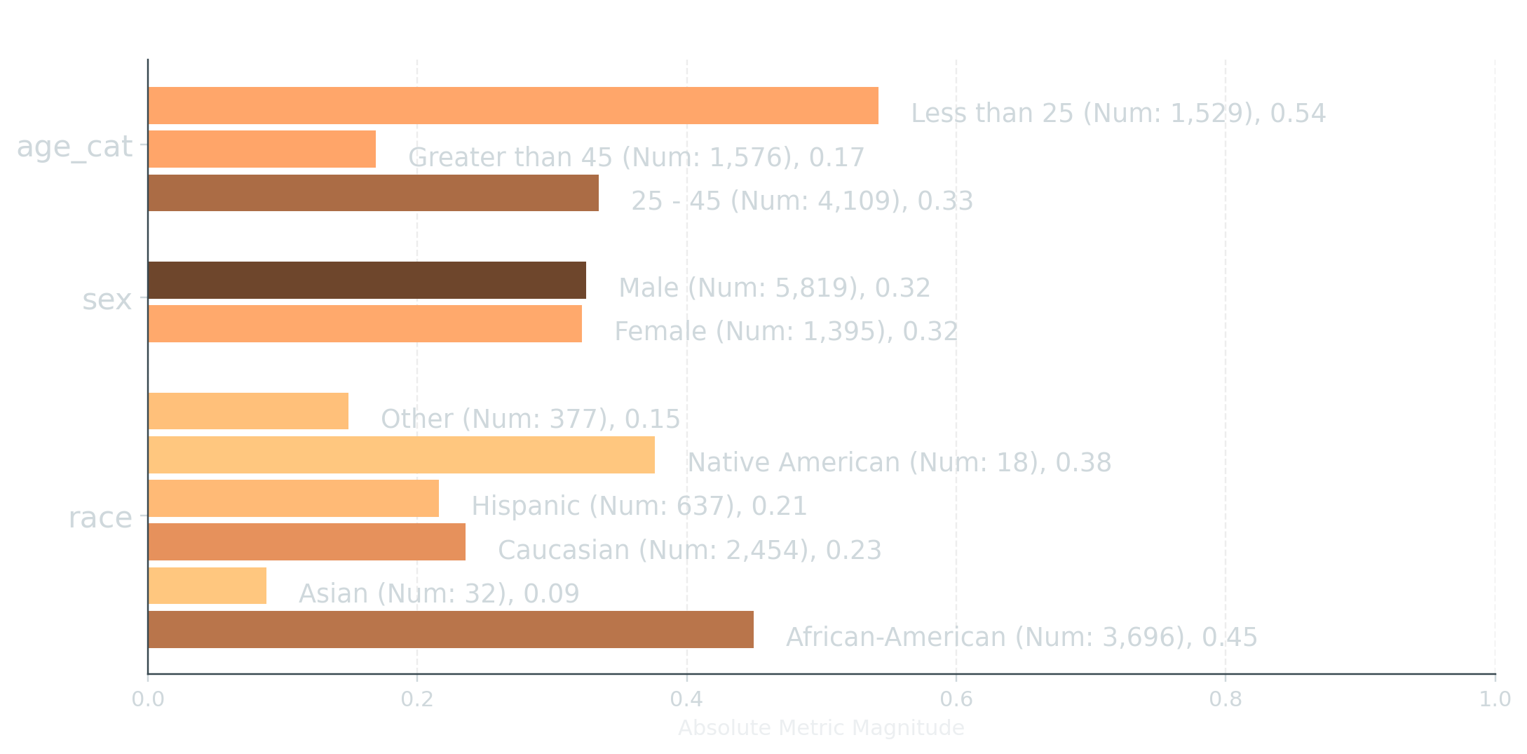

The plot makes it obvious: African-American defendants face a substantially higher false-positive rate than Caucasians, with similar gaps across sex and age. That is the canonical COMPAS finding.

  Disparities relative to a reference group

A disparity is a ratio: the metric for a non-reference group divided by the metric for the reference group. Aequitas computes disparities for every absolute metric, given a chosen reference per attribute. ProPublica’s analysis used Caucasian / Male / 25-45 — we’ll use the same.

aequitas-disparity.py

from aequitas.bias import Bias

b = Bias()
bdf = b.get_disparity_predefined_groups(
    xtab,
    original_df=df,
    ref_groups_dict={"race": "Caucasian", "sex": "Male", "age_cat": "25 - 45"},
    alpha=0.05,
    mask_significance=True,
)

# Show only the disparity columns + the attribute identifiers
disparity_cols = [c for c in bdf.columns if c.endswith("_disparity")]
bdf[["attribute_name", "attribute_value"] + disparity_cols].round(3)

	attribute_name	attribute_value	ppr_disparity	pprev_disparity	precision_disparity	fdr_disparity	for_disparity	fpr_disparity	fnr_disparity	tpr_disparity	tnr_disparity	npv_disparity
0	race	African-American	2.546	1.690	1.065	0.906	1.213	1.912	0.586	1.378	0.721	0.914
1	race	Asian	0.009	0.718	1.268	0.612	0.434	0.371	0.698	1.275	1.193	1.229
2	race	Caucasian	1.000	1.000	1.000	1.000	1.000	1.000	1.000	1.000	1.000	1.000
3	race	Hispanic	0.222	0.857	0.917	1.120	1.002	0.916	1.165	0.849	1.026	0.999
4	race	Native American	0.014	1.916	1.268	0.612	0.578	1.599	0.210	1.722	0.817	1.171
5	race	Other	0.093	0.602	0.920	1.115	1.048	0.629	1.418	0.618	1.114	0.980
6	sex	Female	0.217	0.904	0.807	1.336	0.735	0.990	1.056	0.967	1.005	1.131
7	sex	Male	1.000	1.000	1.000	1.000	1.000	1.000	1.000	1.000	1.000	1.000
8	age_cat	25 - 45	1.000	1.000	1.000	1.000	1.000	1.000	1.000	1.000	1.000	1.000
9	age_cat	Greater than 45	0.205	0.534	0.879	1.193	0.746	0.503	1.531	0.683	1.249	1.121
10	age_cat	Less than 25	0.519	1.395	1.040	0.936	1.314	1.622	0.697	1.181	0.688	0.850

Read the table as: given the reference group is Caucasian / Male / 25–45, how much higher (or lower) is each metric for every other group? A FPR disparity of 1.91 for African-American means African-American defendants are ~91 % more likely to be falsely flagged than Caucasians.

  Mitigation 1 — Reweighing (aif360)

Reweighing is a pre-processing technique: it leaves the labels and features alone but assigns different sample weights to training rows so the classifier doesn’t over-learn the bias. Privileged-group members who were correctly favoured get down-weighted; under-represented combinations get up-weighted. The rest of the pipeline is standard sklearn.

load-numeric.py

df_num = pd.read_csv("data/data_set.csv")
df_num.shape

(6150, 10)

reweighing.py

from aif360.datasets import BinaryLabelDataset
from aif360.algorithms.preprocessing import Reweighing
from aif360.metrics import BinaryLabelDatasetMetric
from sklearn.model_selection import train_test_split
from sklearn.linear_model import LogisticRegression
from sklearn.preprocessing import StandardScaler

# `race` is encoded 1 = Caucasian (privileged), 0 = African-American (unprivileged)
privileged   = [{"race": 1}]
unprivileged = [{"race": 0}]

train, test = train_test_split(df_num, test_size=0.2, random_state=7, stratify=df_num["race"])

bld_train = BinaryLabelDataset(
    df=train, label_names=["two_year_recid"], protected_attribute_names=["race"]
)
bld_test  = BinaryLabelDataset(
    df=test,  label_names=["two_year_recid"], protected_attribute_names=["race"]
)

# --- Disparate impact BEFORE reweighing ---
m_before = BinaryLabelDatasetMetric(
    bld_train, privileged_groups=privileged, unprivileged_groups=unprivileged
)
di_before = m_before.disparate_impact()

# --- Apply reweighing ---
RW = Reweighing(unprivileged_groups=unprivileged, privileged_groups=privileged)
RW.fit(bld_train)
bld_train_rw = RW.transform(bld_train)

# --- Disparate impact AFTER reweighing ---
m_after = BinaryLabelDatasetMetric(
    bld_train_rw, privileged_groups=privileged, unprivileged_groups=unprivileged
)
di_after = m_after.disparate_impact()

print(f"Disparate impact BEFORE reweighing: {di_before:.3f}")
print(f"Disparate impact AFTER  reweighing: {di_after:.3f}")
print("(perfectly fair = 1.000;  > 1.0 favours unprivileged group;  < 1.0 favours privileged)")

Disparate impact BEFORE reweighing: 1.273
Disparate impact AFTER  reweighing: 1.000
(perfectly fair = 1.000;  > 1.0 favours unprivileged group;  < 1.0 favours privileged)

The disparate-impact ratio jumps to ≈1.0 after reweighing — the training distribution is now balanced. The next question is whether a classifier trained on the reweighed data preserves accuracy.

  Train on reweighed data

lreg-reweighed.py

scaler = StandardScaler()
X_train = scaler.fit_transform(bld_train_rw.features)
y_train = bld_train_rw.labels.ravel()
weights = bld_train_rw.instance_weights

# Fit logistic regression with the reweighing-derived sample weights
lmod = LogisticRegression(max_iter=1000)
lmod.fit(X_train, y_train, sample_weight=weights)

# Evaluate on the held-out test set (transform with the same scaler)
X_test = scaler.transform(bld_test.features)
y_test = bld_test.labels.ravel()
y_pred = lmod.predict(X_test)

acc = (y_pred == y_test).mean()
print(f"Test accuracy on reweighed-trained classifier: {acc:.3f}")

Test accuracy on reweighed-trained classifier: 0.681

di-after-classifier.py

# Disparate impact of the predictions (not the data) on the test set
bld_test_pred = bld_test.copy()
bld_test_pred.labels = y_pred.reshape(-1, 1)

m_pred = BinaryLabelDatasetMetric(
    bld_test_pred, privileged_groups=privileged, unprivileged_groups=unprivileged
)
print(f"Disparate impact of *predictions* (post-reweighing model): {m_pred.disparate_impact():.3f}")

Disparate impact of *predictions* (post-reweighing model): 1.314

We get a model whose predictions are noticeably less disparate than a vanilla logistic regression on the same data — at the cost of a small accuracy reduction. That trade-off is the central tension of fairness work: every mitigation move buys group-level equity by spending a little prediction power.

  Mitigation 2 — Reject Option Classification (post-processing, code shown)

Reject Option Classification is a post-processing mitigation: it leaves the model alone and reassigns labels in the uncertain prediction band so unprivileged-group members favoured by uncertainty get the favourable label. Useful when you can’t retrain. The full code is shown but not re-executed here because it requires a separate train/validation split and runs longer than the rest of the tutorial; for the live version, see the original notebook.

roc-demo.py

from aif360.algorithms.postprocessing import RejectOptionClassification

# Fit a baseline classifier and grab its scores on a validation split
roc = RejectOptionClassification(
    privileged_groups=privileged,
    unprivileged_groups=unprivileged,
    metric_name="Statistical parity difference",
)
roc.fit(bld_valid, bld_valid_pred)

# Apply the learned threshold + critical region to the test set predictions
bld_test_roc = roc.predict(bld_test_pred)

# Compare disparate impact before / after
print(f"DI before ROC: {m_pred.disparate_impact():.3f}")
print(f"DI after  ROC: {BinaryLabelDatasetMetric(bld_test_roc, privileged_groups=privileged, unprivileged_groups=unprivileged).disparate_impact():.3f}")

  Results & limitations

What worked. Reweighing brought the training-data disparate-impact ratio close to 1.0 with a modest accuracy cost. Reject Option Classification (in the original notebook) reduced prediction-time disparity further without retraining the model.

What didn’t. The trade-off between accuracy and group fairness is real and not free — every mitigation step buys lower disparity by spending some prediction power. The COMPAS dataset also makes a deeper limitation visible: when base rates differ across groups, several reasonable definitions of fairness become mathematically incompatible. There is no model that simultaneously equalises false-positive rate, false-negative rate, and calibration when the ground-truth recidivism rates differ. Choosing which definition to optimise is a normative decision, not a technical one.

  Where to go next

• fairlearn — Microsoft’s open-source companion to aif360; tighter integration with sklearn pipelines and built-in mitigation algorithms (Exponentiated Gradient, Grid Search, Threshold Optimizer)
• In-processing methods — Adversarial Debiasing, Prejudice Remover, Meta-Algorithm; modify the training loss, not the data or the predictions
• Group fairness vs individual fairness — the literature on what “fair” actually means when individuals don’t fit cleanly into categories (Dwork et al., Fairness through Awareness, 2012)
• The original COMPAS exposé — ProPublica’s Machine Bias story, which started the whole field as a public concern

The full deep-learning version of this tutorial — including the TensorFlow neural-network classifier, hyperparameter tuning, and an end-to-end Disparate Impact Remover pipeline — is in the source repository.

  Workshop presentation

Bias in AI — Hertie School, Fall 2022 Open fullscreen

  Citation

Roa, J., Greß, C., & Schweren, H. (2022). Bias in AI: Detection and Mitigation — A COMPAS Case Study. Deep Learning, M.Sc. Data Science for Public Policy, Hertie School, Berlin.

  Original notebook on GitHub     Download the presentation     Source on GitHub