How We Met Quanteda — Text Analysis with R

Track 01 · Text Analysis & NLP · Tutorial

A hands-on introduction to quanteda built around an unlikely teaching corpus: every line of dialogue from How I Met Your Mother. Covers corpus construction, preprocessing, document-feature matrices, similarity, networks, and collocations.

How We Met Quanteda

November 2022 · Berlin

Roa, J., Fonseca, A., Kraess, A.

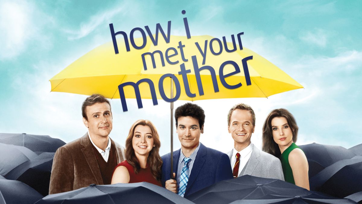
How I Met Your Mother — six seasons of objects, one frame Television corpus · 208 episodes, 2005–2014 A corpus is not a document — it is the arrangement. Five voices over nine years, each measurable by frequency, each locatable by co-occurrence, each distinguishable by what it says most often and least. The tools that read this one read any other with the same keystrokes.

  Objective

This workshop uses the quanteda R package to analyze the television series How I Met Your Mother and walk through the package’s main tools — corpus building, tokenisation, document-feature matrices, similarity & distance, character-frequency tracking, wordclouds, network plots, and multi-word collocations. The point is not the show; the point is that the same pipeline scales to any text data, and a sitcom is a friendlier playground than a parliamentary corpus when you’re learning the API for the first time.

  How I Met Your Mother

Why this corpus

How I Met Your Mother ran for 9 seasons and 208 episodes between 2005 and 2014. A multi-character sitcom with stable principals, recurring secondary characters, and well-defined seasonal arcs is an unusually well-shaped corpus for teaching: the structure (5 anchors + a long tail of recurring names) makes frequency, network, and KWIC analyses produce visibly correct results without forcing the audience to memorise an unfamiliar domain first.

"The story of five friends sitting in their favorite booth at MacLaren's, their lives unfolding in front of each other..."

  Principal Characters

Ted

Josh Radnor

Barney

Neil Patrick Harris

Robin

Cobie Smulders

Marshall

Jason Segel

Lily

Alyson Hannigan

“Some believe HIMYM is Ted’s story. Others think that it is Marshall and Lily’s story. And there’s a whole school of thought that it’s no one else but Barney’s story. We’d like to think it’s all of their stories — there won’t be a Ted without Barney, a Lily without Marshall, and definitely no Robin without a Ted (and Barney too).” — framing taken from the original IDS workshop materials

  Setup

The libraries below cover the full pipeline. The original workshop also used polite, rvest, and httr for the live web-scrape step that produced the corpus — those are not loaded here because the data is already on disk.

• quanteda — core text-analysis API: corpus, tokens, dfm
• quanteda.textplots — wordclouds and network plots
• quanteda.textstats — frequency, similarity, collocations
• readtext — loading plain-text and formatted docs into R
• dplyr · stringr — data wrangling and regex extraction
• ggplot2 · ggrepel — plotting + non-overlapping text labels
• RColorBrewer — categorical and sequential palettes

setup.R

library(quanteda)
library(quanteda.textplots)
library(quanteda.textstats)
library(readtext)
library(stringr)
library(dplyr)
library(ggplot2)
library(ggrepel)
library(RColorBrewer)

# Custom ggplot theme for the dark site — transparent backgrounds so the page
# shows through, light text colours so labels remain readable.
theme_dark_transparent <- function(base_size = 12) {
  theme_minimal(base_size = base_size) %+replace%
    theme(
      plot.background   = element_rect(fill = "transparent", color = NA),
      panel.background  = element_rect(fill = "transparent", color = NA),
      panel.grid.major  = element_line(color = "#37474f"),
      panel.grid.minor  = element_blank(),
      axis.text         = element_text(color = "#cfd8dc"),
      axis.title        = element_text(color = "#eceff1"),
      plot.title        = element_text(color = "#ffffff", face = "bold",
                                       hjust = 0, margin = margin(0, 0, 10, 0)),
      plot.subtitle     = element_text(color = "#b0bec5", hjust = 0),
      plot.caption      = element_text(color = "#78909c", hjust = 0),
      legend.background = element_rect(fill = "transparent", color = NA),
      legend.key        = element_rect(fill = "transparent", color = NA),
      legend.text       = element_text(color = "#cfd8dc"),
      legend.title      = element_text(color = "#eceff1"),
      strip.background  = element_rect(fill = "transparent", color = NA),
      strip.text        = element_text(color = "#eceff1")
    )
}
theme_set(theme_dark_transparent())

# par() defaults for base-R plots (dendrograms, wordclouds, networks) so they
# match the light-on-transparent palette used by ggplot.
par_dark <- function() {
  par(
    bg       = NA,
    col.axis = "#cfd8dc",
    col.lab  = "#eceff1",
    col.main = "#ffffff",
    col.sub  = "#b0bec5",
    fg       = "#cfd8dc"
  )
}

# Tutorial-wide palette — Material Design 300/400 brightness range.
# All colours stay readable on the dark page; first one is the site accent.
tutorial_pal <- c(
  blue   = "#64B5F6",
  coral  = "#FF8A65",
  mint   = "#81C784",
  gold   = "#FFCA28",
  purple = "#BA68C8",
  cyan   = "#4DD0E1",
  pink   = "#F48FB1",
  amber  = "#FFB74D"
)

# Per-character colours for the principal-cast plots (5 named lines).
principal_colors <- c(
  Ted      = "#64B5F6",
  Marshall = "#81C784",
  Lily     = "#F48FB1",
  Robin    = "#FFCA28",
  Barney   = "#FF8A65"
)

# Path to the scraped HIMYM scripts. The directory holds 208 episode .txt
# files named like "how-i-met-your-mother_04e23.txt".
texts_dir <- "texts/how-i-met-your-mother"

# Principal cast: the five main characters who anchor the show.
principals <- c("Ted", "Marshall", "Lily", "Robin", "Barney")

  How the corpus was sourced (web-scrape)

The 208 .txt files were produced once with a polite scrape of SpringfieldSpringfield.co.uk — a public archive of TV transcripts. The code below is from the original notebook and is shown for reference only; we don’t re-execute it on every render. If you ever need to refresh the corpus, this is the pattern.

scrape-demo.R

# library(rvest); library(polite); library(httr)
v_tv_show <- "how-i-met-your-mother"
v_url_web <- "http://www.springfieldspringfield.co.uk/"

# Bow before scraping — checks robots.txt and crawl delay
session_information <- bow(v_url_web)

# Identify yourself when scraping (good citizenship)
v_url <- paste0(v_url_web, "episode_scripts.php?tv-show=", v_tv_show)
rvest_himym <- session(
  v_url,
  add_headers(`From` = "you@example.com",
              `UserAgent` = R.Version()$version.string)
)

# Discover episode URLs, then loop and save each script as a .txt
html_url_scrape <- rvest_himym |> read_html(v_url)
hrefs <- html_nodes(html_url_scrape, ".season-episode-title") |> html_attr("href")

for (x in hrefs) {
  Sys.sleep(runif(1, 0, 1))   # be polite — random pause between requests
  text_html <- read_html(paste(v_url_web, x, sep = "/")) |>
    html_nodes(".scrolling-script-container") |>
    html_text()
  # ... write each episode as its own .txt under texts/how-i-met-your-mother/
}

Why the scrape isn’t live in this tutorial. Two reasons. First, web-scraping inside a tutorial render is fragile — if the source page changes structure or rate-limits, your whole site build breaks. Second, the politeness pattern (Sys.sleep, identification headers, bow) is the point of this section: it teaches the how, not the data acquisition itself. Run the loop once locally; commit the resulting .txt files; let chunks downstream read from disk.

1. Load the episode scripts

readtext() is the canonical companion to quanteda for getting text off disk. We point it at the directory and let it discover every .txt file. The filenames carry the season and episode (04e23 → Season 4, Episode 23), so we parse them out as document-level variables.

load-scripts.R

scripts <- readtext(file.path(texts_dir, "*.txt"))

scripts <- scripts |>
  mutate(
    season  = as.integer(str_extract(doc_id, "(?<=_)\\d+(?=e)")),
    episode = as.integer(str_extract(doc_id, "(?<=e)\\d+(?=\\.txt)"))
  )

dim(scripts)
#> [1] 208   4
head(scripts |> select(doc_id, season, episode), 5)
#> readtext object consisting of 5 documents and 1 docvar.
#> # A data frame: 5 x 4
#>   doc_id                          season episode text     
#> * <chr>                            <int>   <int> <chr>    
#> 1 how-i-met-your-mother_01e01.txt      1       1 "\"\"..."
#> 2 how-i-met-your-mother_01e02.txt      1       2 "\"\"..."
#> 3 how-i-met-your-mother_01e03.txt      1       3 "\"\"..."
#> 4 how-i-met-your-mother_01e04.txt      1       4 "\"\"..."
#> 5 how-i-met-your-mother_01e05.txt      1       5 "\"\"..."

208 episodes loaded, season + episode attached. That’s enough metadata to do the per-season comparisons, dendrograms, and character-frequency tracking that follow.

2. From text to corpus

A corpus is text + docvars in one object — text under one column, episode metadata under others.

A quanteda corpus is text plus docvars in one object. Every column besides the text becomes a document-level variable.

corpus.R

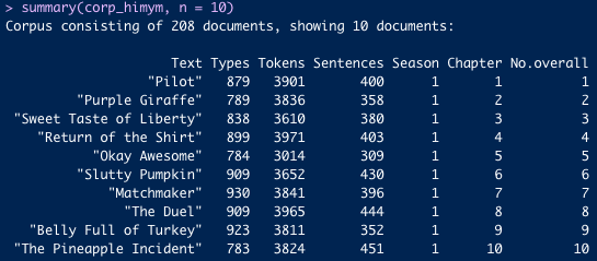
corp_himym <- corpus(scripts, docid_field = "doc_id", text_field = "text")
docnames(corp_himym) <- paste0("S", scripts$season, "_E", scripts$episode)

corp_himym
#> Corpus consisting of 208 documents and 2 docvars.
#> S1_E1 :
#> ""x" "                      OLDER TED: Kids, I'm gonna tell y..."
#> 
#> S1_E2 :
#> ""x" "                      - OLDER TED: Okay, where was I? -..."
#> 
#> S1_E3 :
#> ""x" "                      S Sy Syn Sync Sync b OLDER TED: S..."
#> 
#> S1_E4 :
#> ""x" "                      OLDER TED: Kids, when you're sing..."
#> 
#> S1_E5 :
#> ""x" "                      OLDER TED: So, kids, would you li..."
#> 
#> S1_E6 :
#> ""x" "                      OLDER TED: You know how Aunt Robi..."
#> 
#> [ reached max_ndoc ... 202 more documents ]
summary(corp_himym, n = 5)
#> Corpus consisting of 208 documents, showing 5 documents:
#> 
#>   Text Types Tokens Sentences season episode
#>  S1_E1   879   3901       400      1       1
#>  S1_E2   789   3836       358      1       2
#>  S1_E3   838   3610       380      1       3
#>  S1_E4   899   3971       403      1       4
#>  S1_E5   784   3015       309      1       5

The first five episodes are around 4,000–5,000 tokens and 350–500 sentences each — consistent with a 22-minute sitcom script.

3. From corpus to tokens

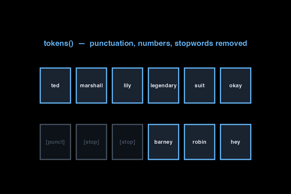
Tokens break a document into units. Almost every preprocessing decision lives at this step.

Tokenisation is where preprocessing decisions live. Punctuation off, numbers off, symbols off, lowercase, stopwords removed — order matters (always remove stopwords after lowercasing).

tokens.R

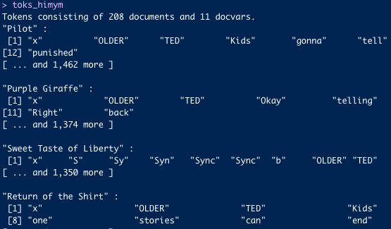
toks <- corp_himym |>
  tokens(
    remove_punct   = TRUE,
    remove_numbers = TRUE,
    remove_symbols = TRUE
  ) |>
  tokens_tolower() |>
  tokens_remove(stopwords("english"))

toks
#> Tokens consisting of 208 documents and 2 docvars.
#> S1_E1 :
#>  [1] "x"          "older"      "ted"        "kids"       "gonna"     
#>  [6] "tell"       "incredible" "story"      "story"      "met"       
#> [11] "mother"     "punished"  
#> [ ... and 1,464 more ]
#> 
#> S1_E2 :
#>  [1] "x"            "older"        "ted"          "okay"         "telling"     
#>  [6] "us"           "met"          "mom"          "excruciating" "detail"      
#> [11] "right"        "back"        
#> [ ... and 1,375 more ]
#> 
#> S1_E3 :
#>  [1] "x"     "s"     "sy"    "syn"   "sync"  "sync"  "b"     "older" "ted"  
#> [10] "one"   "night" "met"  
#> [ ... and 1,351 more ]
#> 
#> S1_E4 :
#>  [1] "x"                  "older"              "ted"               
#>  [4] "kids"               "single"             "looking"           
#>  [7] "happily-ever-after" "one"                "stories"           
#> [10] "can"                "end"                "way"               
#> [ ... and 1,481 more ]
#> 
#> S1_E5 :
#>  [1] "x"     "older" "ted"   "kids"  "like"  "hear"  "story" "time"  "went" 
#> [10] "deaf"  "even"  "ask"  
#> [ ... and 1,140 more ]
#> 
#> S1_E6 :
#>  [1] "x"         "older"     "ted"       "know"      "aunt"      "robin's"  
#>  [7] "big"       "fan"       "halloween" "always"    "dressing"  "crazy"    
#> [ ... and 1,405 more ]
#> 
#> [ reached max_ndoc ... 202 more documents ]

Preprocessing is a modeling choice, not a default. Removing stopwords helps when content words are what you care about; it hurts when style is the question. Lowercasing erases proper-noun information. There is no universally correct setting — it depends on the question.

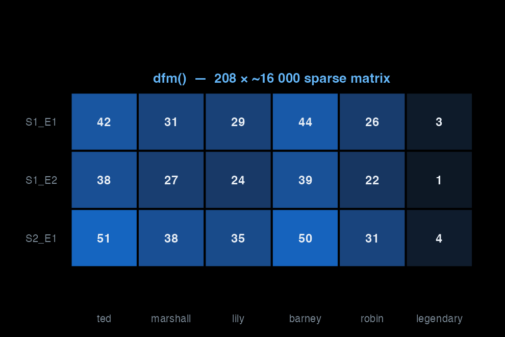
4. From tokens to a dfm

The DFM is the workhorse: rows = documents, columns = features, cells = counts.

dfm.R

dfm_himym <- dfm(toks)
dfm_himym
#> Document-feature matrix of: 208 documents, 20,711 features (96.69% sparse) and 2 docvars.
#>        features
#> docs    x older ted kids gonna tell incredible story met mother
#>   S1_E1 1     1  22    3    22    6          1     7  11      1
#>   S1_E2 1     5  30    2    19    1          1     1  10      0
#>   S1_E3 1     3  27    1    15    6          0     2   1      1
#>   S1_E4 1     5  14    1    15    4          0     6   0      0
#>   S1_E5 1     3   9    2    11    4          0     5   0      0
#>   S1_E6 1     1  16    0    15    1          0     3   4      0
#> [ reached max_ndoc ... 202 more documents, reached max_nfeat ... 20,701 more features ]

A 208 × ~16,000 sparse matrix. Most cells are zero (most words don’t appear in most episodes), which is exactly what Matrix::sparseMatrix is for.

  The workflow at a glance

1 · Text208 raw script .txt files on disk

2 · Corpus`corpus()` — text + season + episode

3 · Tokens`tokens()` — words + preprocessing

4 · DFM`dfm()` — document × feature counts

5 · Analysisfrequency, KWIC, similarity, networks, collocations

Every quanteda pipeline you read in the wild is a variation on these five steps. The interesting decisions live at steps 2 and 3.

The pipeline, in motion

Scroll to see the three objects — corpus, tokens, DFM — and what each transformation discards.

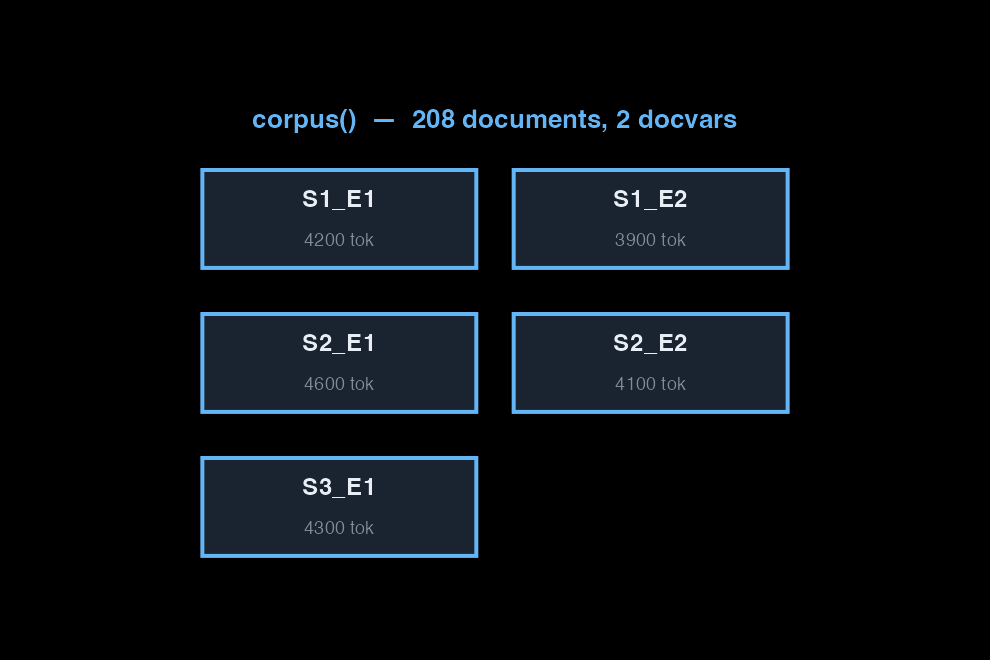
corpus() wraps raw text and metadata into one object. Each document is a row: the text in one column, season and episode number in the others. No words have been touched yet.

tokens() breaks each document into units and applies preprocessing rules. Punctuation, numbers, and stopwords are removed at this step. The greyed tiles are discarded — they never enter the matrix.

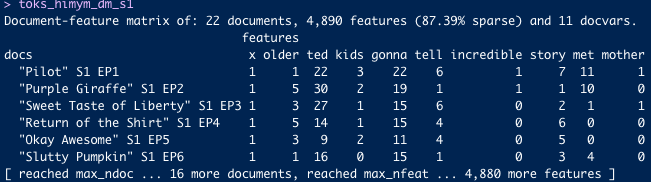
dfm() counts how often each remaining feature appears in each document. Rows are documents, columns are features, cells are counts. Most cells are zero — this is a sparse matrix.

  Top features

topfeatures.R

topfeatures(dfm_himym, n = 25)
#>     just       oh     know      ted     like     okay     yeah    right 
#>     4553     4023     3646     3006     2847     2716     2632     2614 
#>      get      one       go     well      hey   barney    gonna      got 
#>     2563     2190     2105     2083     2037     2028     2000     1898 
#>      now    robin      can marshall     want     lily   really    think 
#>     1856     1835     1809     1807     1766     1745     1654     1525 
#>    going 
#>     1494

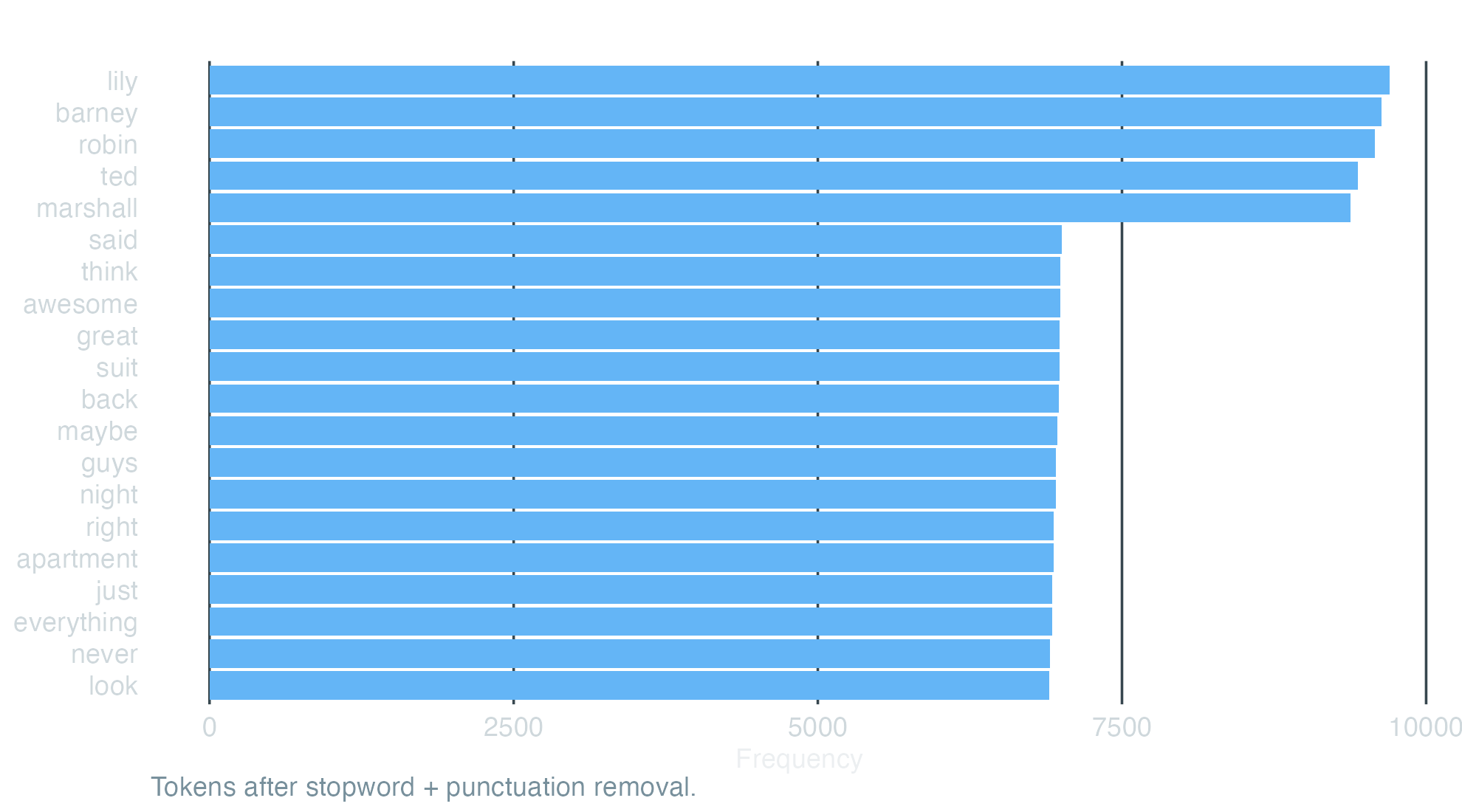
Character names dominate, as you would expect from a multi-character sitcom. quanteda.textstats gives the same view as a tibble we can plot.

freq-plot.R

freq <- textstat_frequency(dfm_himym, n = 20)

ggplot(freq, aes(x = reorder(feature, frequency), y = frequency)) +
  geom_col(fill = "#64B5F6") +
  coord_flip() +
  labs(
    x = NULL, y = "Frequency",
    title = "Top 20 tokens — HIMYM corpus (208 episodes)",
    caption = "Tokens after stopword + punctuation removal."
  ) +
  theme_dark_transparent() +
  theme(panel.grid.major.y = element_blank())

  Wordcloud — overall

wordcloud.R

set.seed(2026)
par_dark()
textplot_wordcloud(
  dfm_himym,
  max_words = 80,
  min_count = 30,
  color = c("#64B5F6", "#90CAF9", "#42A5F5", "#1E88E5", "#1565C0")
)

  Keywords-in-context (KWIC)

KWIC pulls every occurrence of a target word with its surrounding context — the single most useful sanity check in the package. The window controls how many tokens of context show on each side.

kwic-legendary.R

kwic(toks, pattern = "legendary", window = 3) |>
  head(8)
#> Keyword-in-context with 8 matches.                                                                        
#>   [S1_E3, 62]   meet ladies gonna | legendary | phone-five older ted    
#>  [S1_E3, 148] peace suckers right | legendary | plan first gotta        
#>  [S1_E3, 216] sketchy trust gonna | legendary | say legendary okay      
#>  [S1_E3, 218] gonna legendary say | legendary | okay liberal word       
#>  [S1_E3, 222]   okay liberal word | legendary | building igloo central  
#>  [S1_E3, 228]  central park gonna | legendary | snowsuit ted ted        
#>  [S1_E3, 418]     us philly gonna | legendary | man wish guys           
#>  [S1_E3, 874]     half word dairy | legendary | legendary sounds awesome

kwic-suit.R

kwic(toks, pattern = "suit", window = 3) |>
  head(8)
#> Keyword-in-context with 8 matches.                                                             
#>  [S1_E1, 128] meet bar minutes | suit | hey suit just        
#>  [S1_E1, 130] minutes suit hey | suit | just say suit        
#>  [S1_E1, 133]    suit just say | suit | wish put suit        
#>  [S1_E1, 136]    suit wish put | suit | one time blazer      
#>  [S1_E1, 182]   lose goatee go | suit | wearing suit lesson  
#>  [S1_E1, 184]  go suit wearing | suit | lesson two get       
#>  [S1_E1, 188]   lesson two get | suit | suits cool exhibit   
#>  [S1_E1, 422] exactly guy even | suit | plus marshall's found

A 3-token window is enough to verify that the matches are the senses you expect.

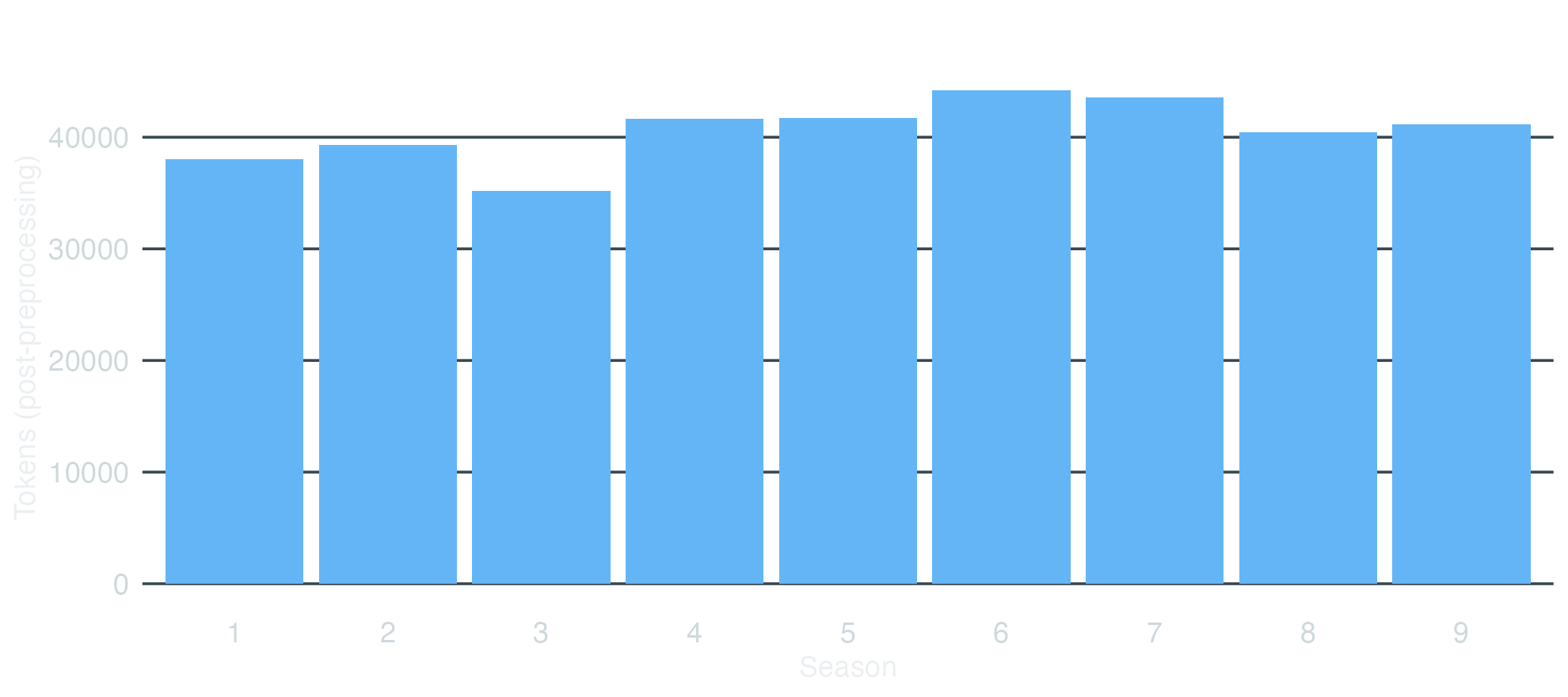
  Token volume per season

tokens-by-season.R

tokens_by_season <- ntoken(dfm_himym) |>
  tibble::enframe(name = "doc", value = "tokens") |>
  mutate(season = scripts$season) |>
  group_by(season) |>
  summarise(total_tokens = sum(tokens), episodes = n(), .groups = "drop")

tokens_by_season
#> # A tibble: 9 x 3
#>   season total_tokens episodes
#>    <int>        <int>    <int>
#> 1      1        31219       22
#> 2      2        31340       22
#> 3      3        28147       20
#> 4      4        33433       24
#> 5      5        36307       24
#> 6      6        34496       24
#> 7      7        35869       24
#> 8      8        36962       24
#> 9      9        41066       24

ggplot(tokens_by_season, aes(x = factor(season), y = total_tokens)) +
  geom_col(fill = "#64B5F6") +
  labs(x = "Season", y = "Tokens (post-preprocessing)",
       title = "Token volume per season") +
  theme_dark_transparent() +
  theme(panel.grid.major.x = element_blank())

  Episode clustering (Season 1)

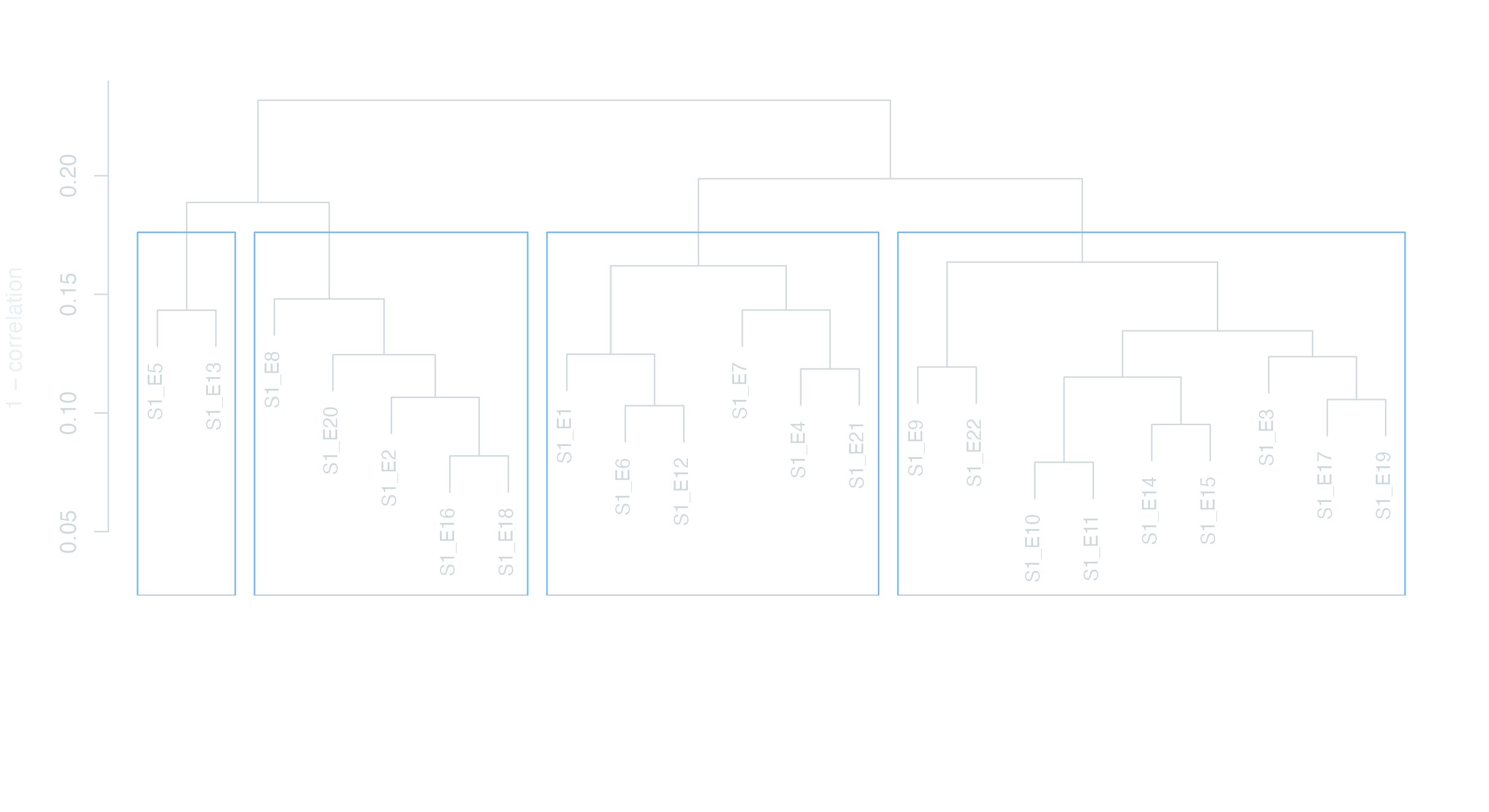
Similarity

textstat_simil() computes pairwise similarity between documents. Most useful at the season level — across 208 episodes the matrix gets unwieldy, but for the 22 episodes of Season 1 we can read the structure off a dendrogram. Cluster the similarity matrix with hclust(), plot as a tree.

similarity-s1.R

dfm_s1 <- dfm_subset(dfm_himym, scripts$season == 1)

simil_s1 <- textstat_simil(dfm_s1, method = "correlation")

clust_s1 <- hclust(as.dist(1 - as.matrix(simil_s1)))

par_dark(); par(mar = c(8, 4, 3, 2))
plot(clust_s1,
     main = "HIMYM Season 1 — episode similarity",
     xlab = "", sub = "", ylab = "1 − correlation",
     cex = 0.85)
rect.hclust(clust_s1, k = 4, border = "#64B5F6")

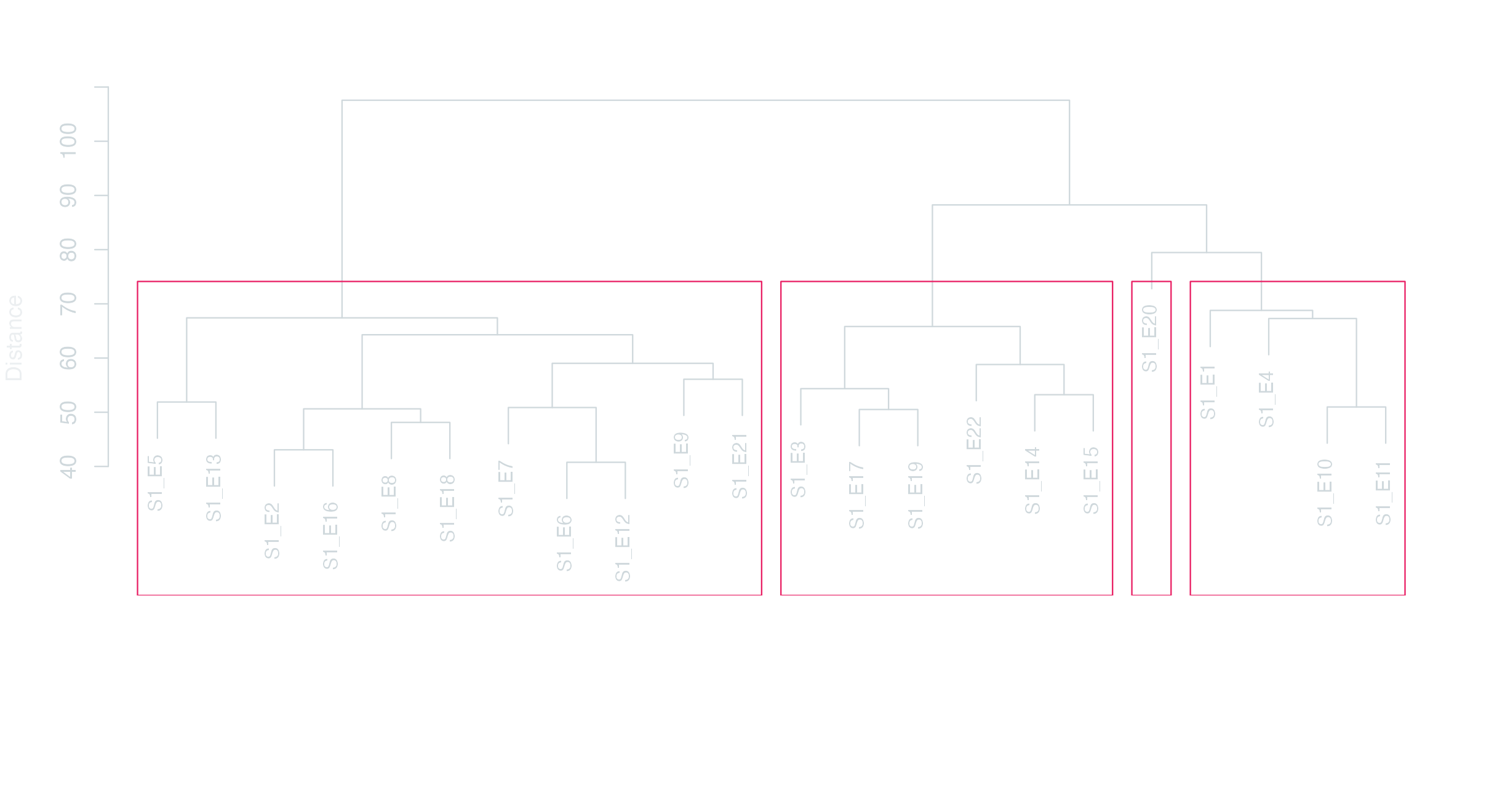
Distance

textstat_dist() is the inverse — how different are episodes? Same dendrogram approach, different metric.

distance-s1.R

dist_s1 <- textstat_dist(dfm_s1, method = "euclidean")

clust_dist_s1 <- hclust(as.dist(as.matrix(dist_s1)))

par_dark(); par(mar = c(8, 4, 3, 2))
plot(clust_dist_s1,
     main = "HIMYM Season 1 — episode distance (Euclidean)",
     xlab = "", sub = "", ylab = "Distance",
     cex = 0.85)
rect.hclust(clust_dist_s1, k = 4, border = "#E91E63")

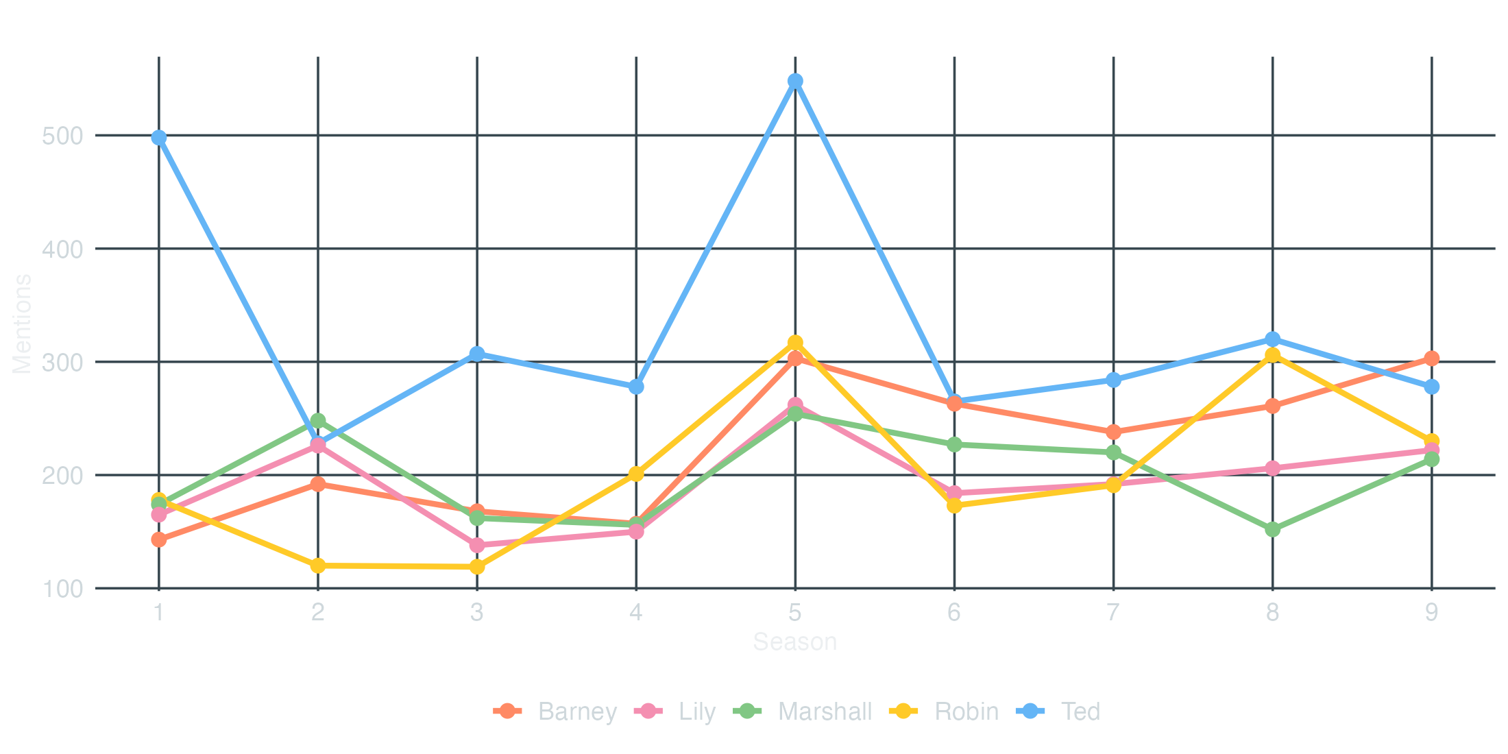
  Principal characters by season

How often each principal is named per season. We tokenise the corpus without lowercasing so we can match capitalised first names directly, keep only the principal cast, group by season, and turn it into a DFM.

principal-frequency.R

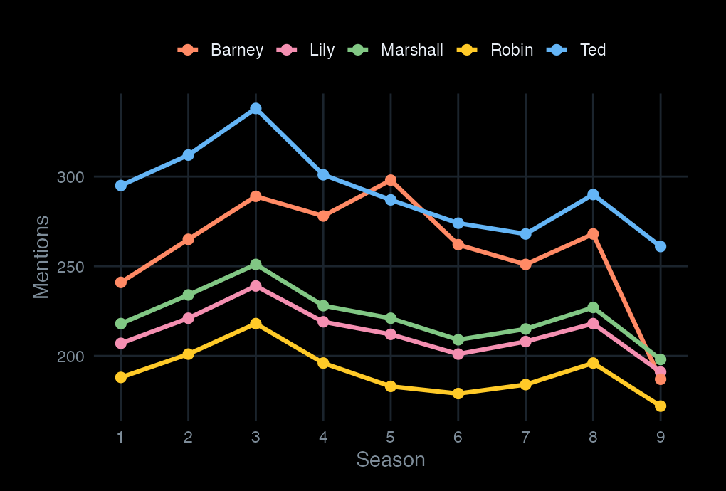
docvars(corp_himym, "season") <- scripts$season

toks_named <- corp_himym |>
  tokens(remove_punct = TRUE, remove_numbers = TRUE, remove_symbols = TRUE)

dfm_principals <- toks_named |>
  tokens_keep(principals) |>
  tokens_group(groups = season) |>
  dfm()

freq_principals <- textstat_frequency(dfm_principals, groups = 1:9) |>
  as_tibble() |>
  mutate(season = as.integer(group),
         character = str_to_title(feature))

freq_principals |> head(10)
#> # A tibble: 10 x 7
#>    feature  frequency  rank docfreq group season character
#>    <chr>        <dbl> <dbl>   <dbl> <chr>  <int> <chr>    
#>  1 ted            498     1       1 1          1 Ted      
#>  2 robin          178     2       1 1          1 Robin    
#>  3 marshall       174     3       1 1          1 Marshall 
#>  4 lily           165     4       1 1          1 Lily     
#>  5 barney         143     5       1 1          1 Barney   
#>  6 marshall       248     1       1 2          2 Marshall 
#>  7 ted            228     2       1 2          2 Ted      
#>  8 lily           226     3       1 2          2 Lily     
#>  9 barney         192     4       1 2          2 Barney   
#> 10 robin          120     5       1 2          2 Robin

ggplot(freq_principals,
       aes(x = season, y = frequency, color = character, group = character)) +
  geom_line(linewidth = 1.3) +
  geom_point(size = 2.8) +
  scale_color_manual(values = principal_colors) +
  scale_x_continuous(breaks = 1:9) +
  labs(x = "Season", y = "Mentions",
       title = "Mentions of principal characters by season",
       color = NULL) +
  theme_dark_transparent() +
  theme(legend.position = "bottom",
        panel.grid.minor = element_blank())

Character arcs, in motion

Scroll to read each character’s presence across the nine seasons.

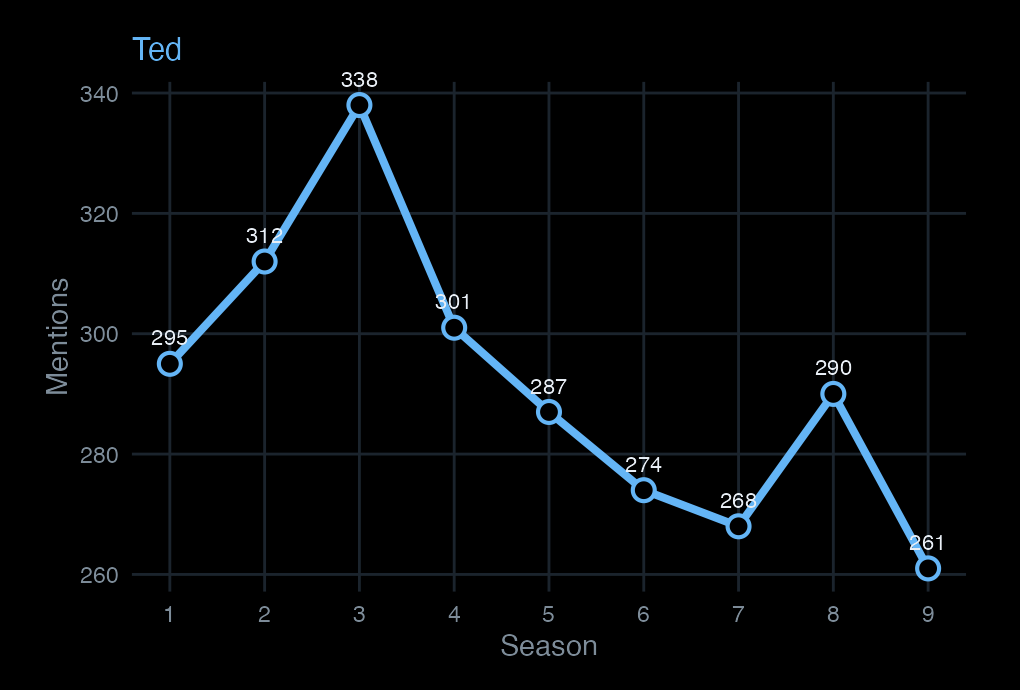
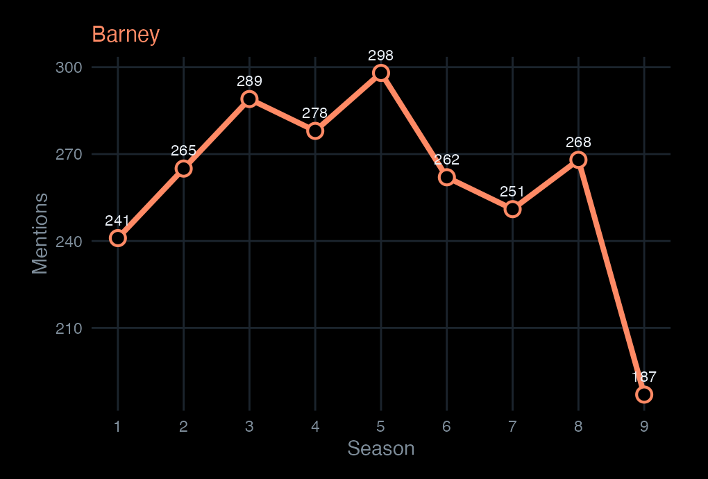
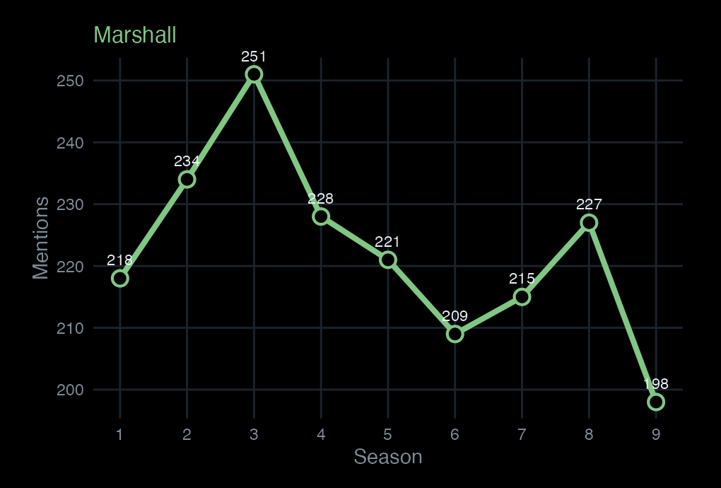
Five characters, nine seasons. This is what a frequency count measures: presence in dialogue, not screen time or plot centrality.

Ted is the narrator’s subject — consistently the most-named character, with a mild dip in Seasons 6–7 where secondary storylines expand.

Barney rises through Season 5 (the year he marries) and drops sharply in Season 9 — the final season compresses his arc into a single weekend.

Marshall runs steady throughout. His mention frequency correlates with the show’s ensemble balance — when Marshall is absent from a storyline, the count drops; when he anchors one, it spikes.

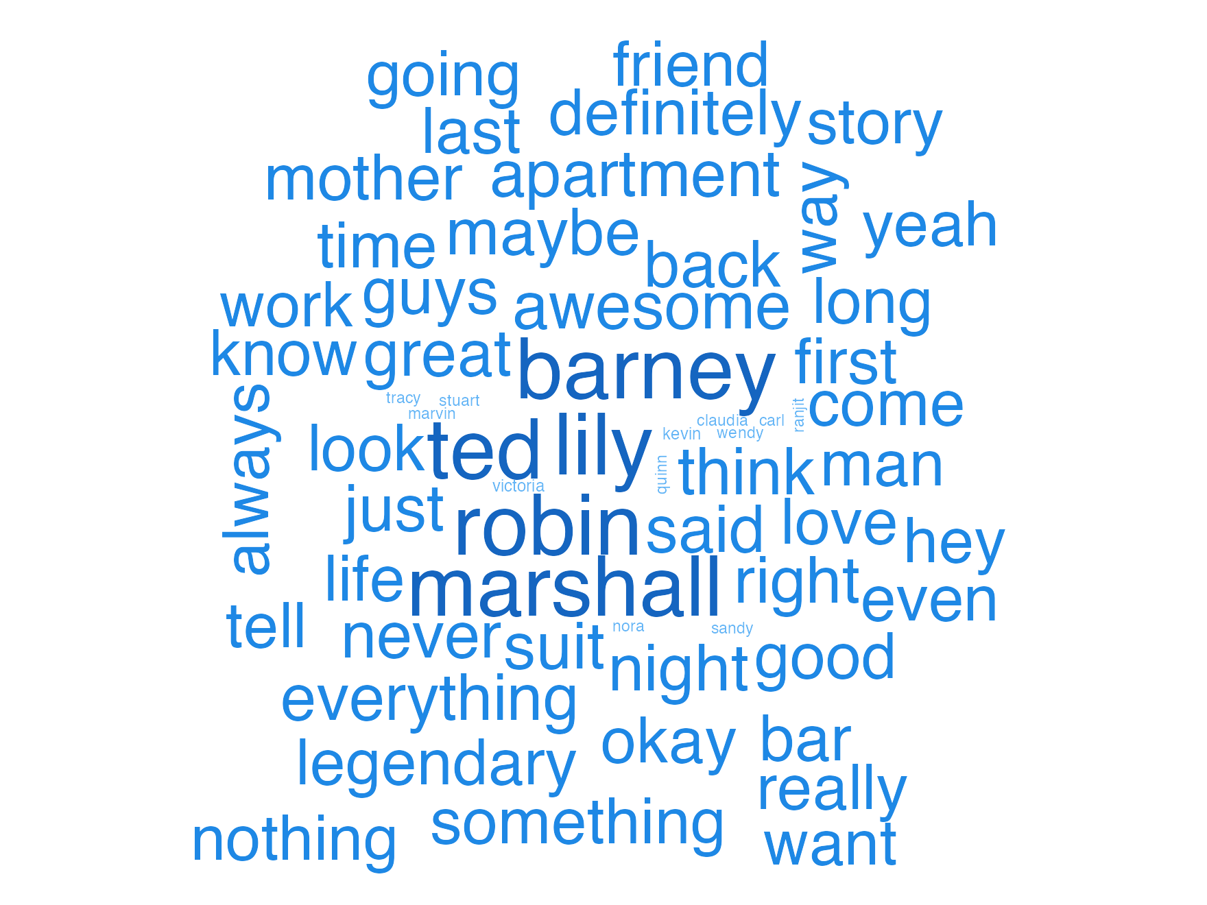
  Character wordclouds

Principal cast

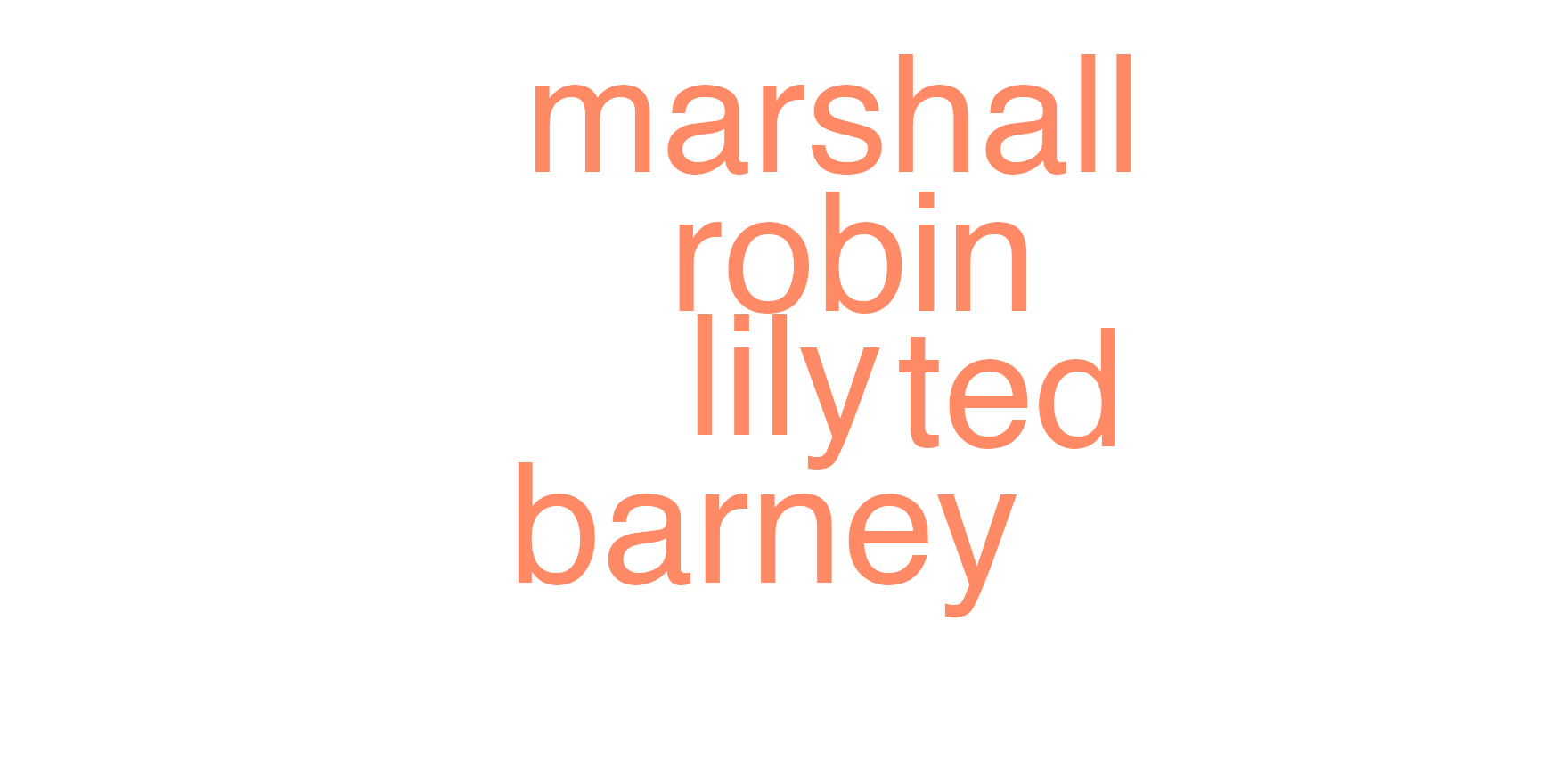
A wordcloud restricted to the five principals: size scales with how often each is named across the whole show.

principal-wordcloud.R

toks_principal_only <- toks_named |> tokens_keep(principals)
dfm_principal_only  <- dfm(toks_principal_only)

set.seed(101)
par_dark()
textplot_wordcloud(
  dfm_principal_only,
  rotation = 0.25,
  min_size = 1.6, max_size = 9,
  color = unname(principal_colors)
)

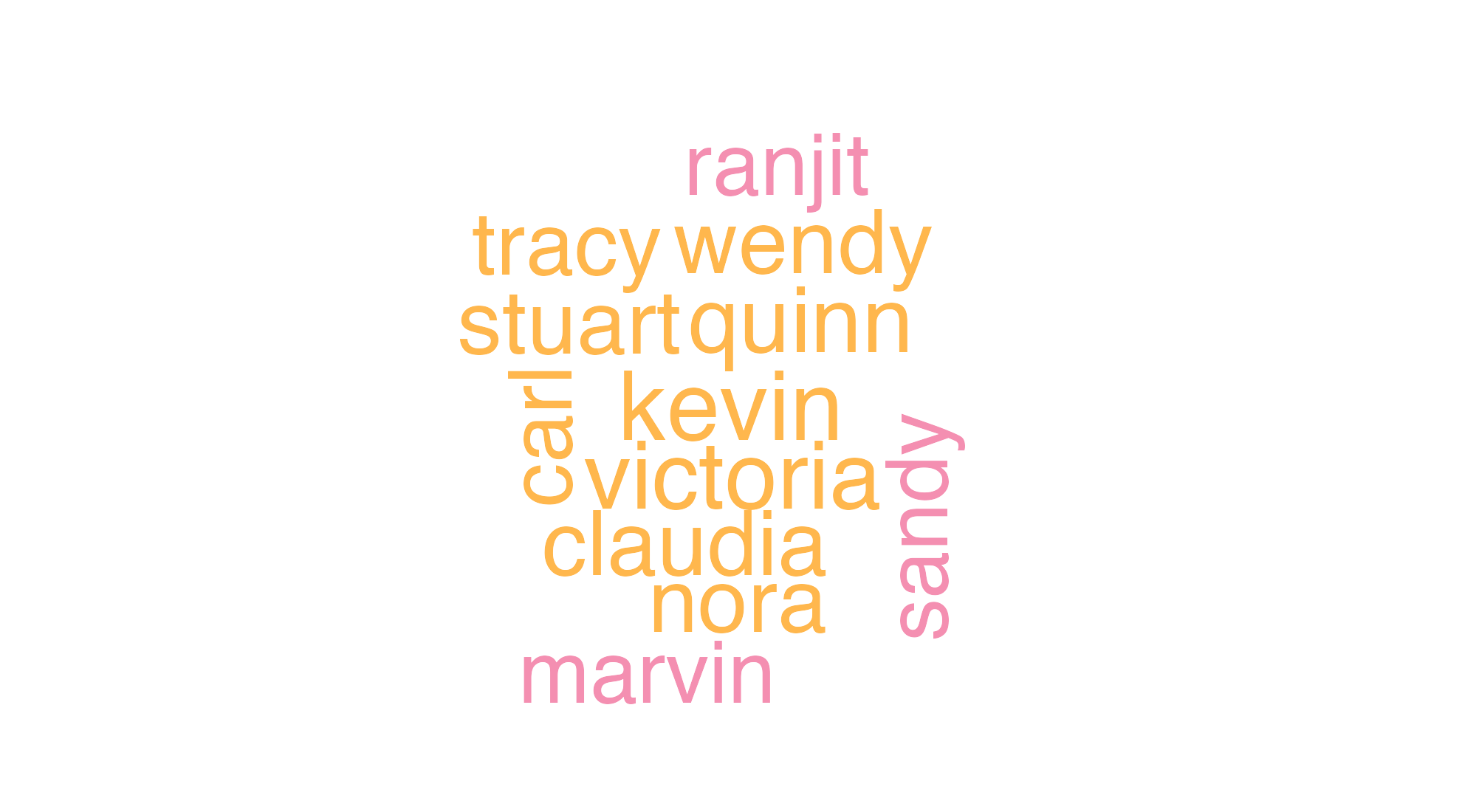
Secondary cast

Secondary characters: a pre-curated set of named recurring characters from across the show, with the principals removed. We need a list of names — the original workshop scraped them from Wikipedia; here we hardcode a representative set so the chunk is reproducible without a network call.

secondary-wordcloud.R

secondary <- c("Tracy", "Marvin", "Loretta", "Wendy", "Carl", "Ranjit",
               "Sandy", "James", "Patrice", "Stella", "Victoria", "Zoey",
               "Quinn", "Don", "Stuart", "Claudia", "Punchy",
               "Tony", "Nora", "Kevin", "Scooter", "Marcus", "Penelope",
               "Mickey", "Judy", "Virginia", "Daphne", "Becky", "Trudy")

toks_secondary <- toks_named |>
  tokens_keep(secondary) |>
  tokens_remove(principals)

dfm_secondary <- dfm(toks_secondary)

set.seed(102)
par_dark()
textplot_wordcloud(
  dfm_secondary,
  rotation = 0.25,
  min_size = 1.0, max_size = 5,
  min_count = 5,
  color = unname(tutorial_pal)
)

  Character co-occurrence networks

Feature co-occurrence matrix

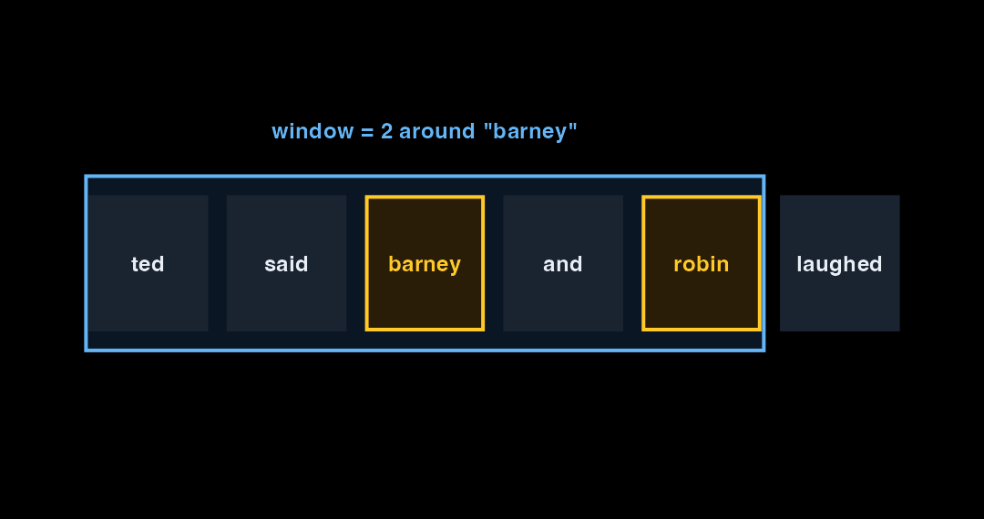
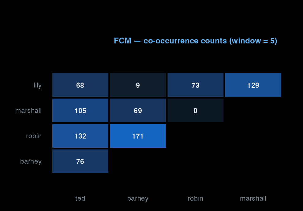
To see who shares scenes with whom, we need a feature co-occurrence matrix (FCM). The window controls what counts as “near” — a 5-token window is the workshop default. We restrict to a small fixed character vocabulary so the matrix is small and the network plots are legible.

character-fcm.R

character_vocab <- str_to_lower(c(principals, secondary))

toks_chars <- toks_named |>
  tokens_tolower() |>
  tokens_keep(character_vocab)

fcm_chars <- fcm(toks_chars, context = "window", window = 5, tri = FALSE)

# `topfeatures()` was deprecated for FCM in quanteda 4.0 — use rowSums + sort
char_totals <- sort(rowSums(fcm_chars), decreasing = TRUE)

dim(fcm_chars)
#> [1] 34 34
head(char_totals, 10)
#>      ted   barney    robin marshall     lily     zoey   stella   marvin 
#>    28441    19072    17484    17099    16609     1464     1435     1251 
#> victoria    james 
#>     1056      891

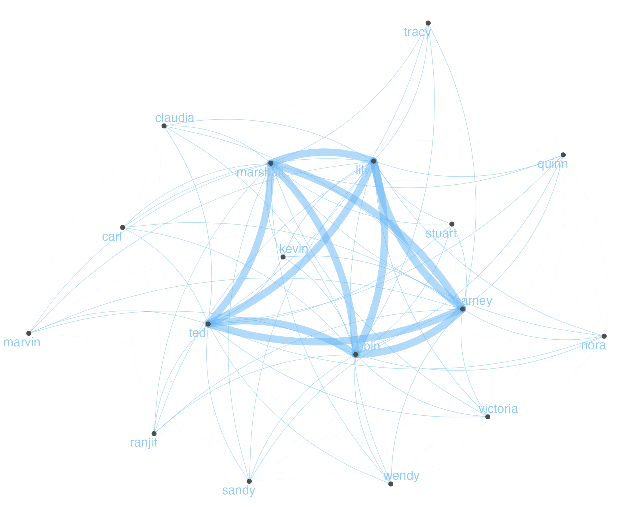
Top 30 characters

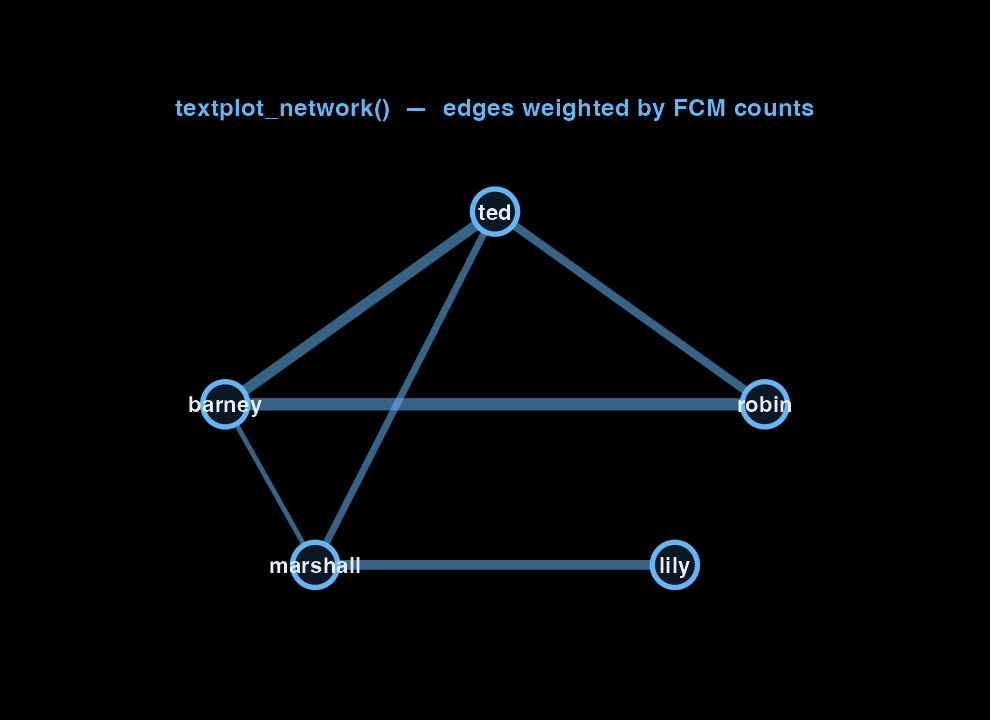
textplot_network() lays the FCM out as a graph: nodes are characters, edges weighted by co-occurrence.

network-30.R

top30 <- names(char_totals)[1:30]

set.seed(100)
par_dark()
textplot_network(
  fcm_select(fcm_chars, top30),
  edge_color = "#64B5F6",
  edge_size = 4,
  vertex_labelcolor = "#90CAF9",
  omit_isolated = TRUE,
  min_freq = 0.1
)

Ted-centred

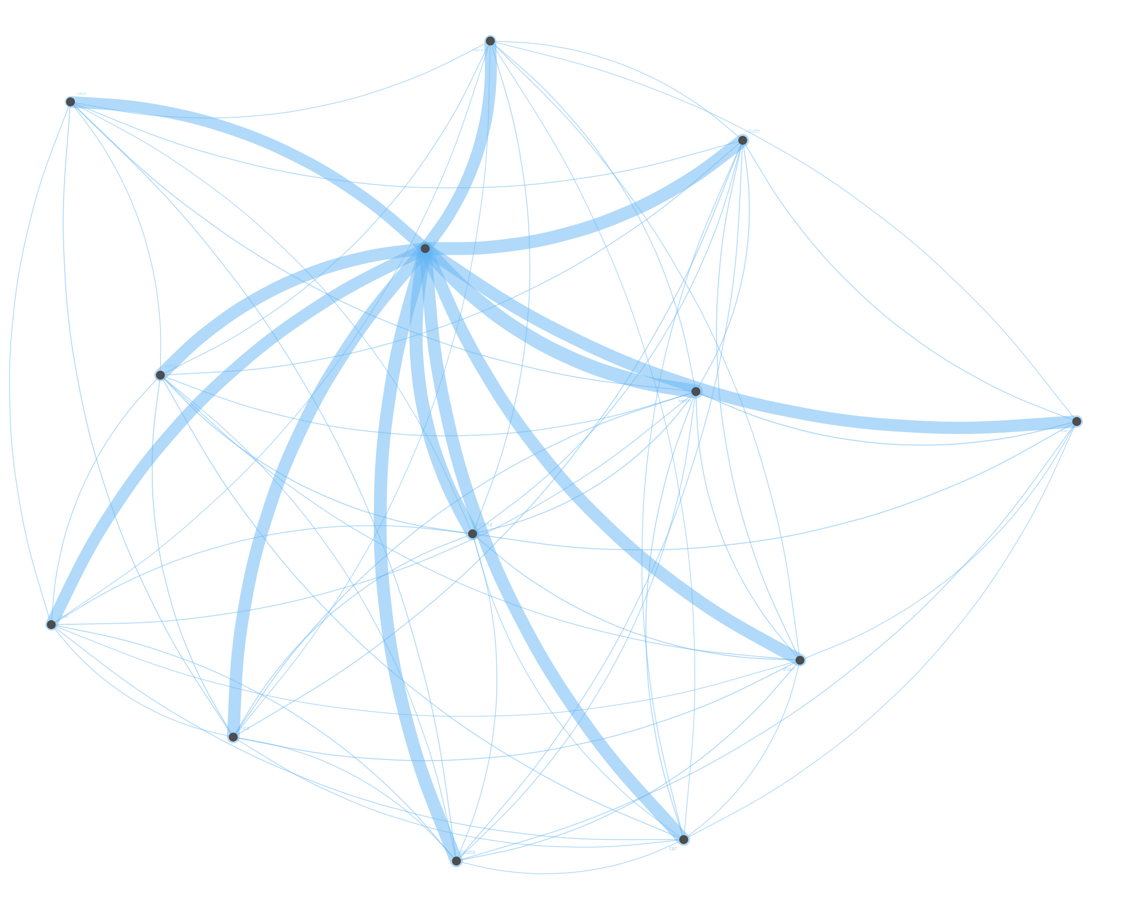
A different question: who shows up in scenes with Ted? We remove the other principals from the corpus first, build a fresh FCM, and weight Ted’s label larger so the centre is unambiguous.

network-ted.R

toks_ted <- toks_chars |>
  tokens_remove(c("marshall", "lily", "barney", "robin"))

fcm_ted <- fcm(toks_ted, context = "window", window = 5, tri = FALSE)

ted_totals <- sort(rowSums(fcm_ted), decreasing = TRUE)
top_ted <- names(ted_totals)[1:30]

vertex_size <- fcm_select(fcm_ted, pattern = top_ted)
weights <- rowSums(vertex_size) / min(rowSums(vertex_size))
weights["ted"] <- weights["ted"] / 15

set.seed(100)
par_dark()
textplot_network(
  fcm_select(fcm_ted, top_ted),
  edge_color = "#64B5F6",
  edge_size = 4,
  vertex_labelcolor = "#90CAF9",
  vertex_labelsize = weights,
  omit_isolated = TRUE,
  min_freq = 0.1
)

  Multi-word collocations (Season 1)

textstat_collocations() finds adjacent fixed-length phrases that appear together more than chance — multi-word expressions, named entities, catch-phrases. We run it on Season 1 to keep the output focused.

collocations.R

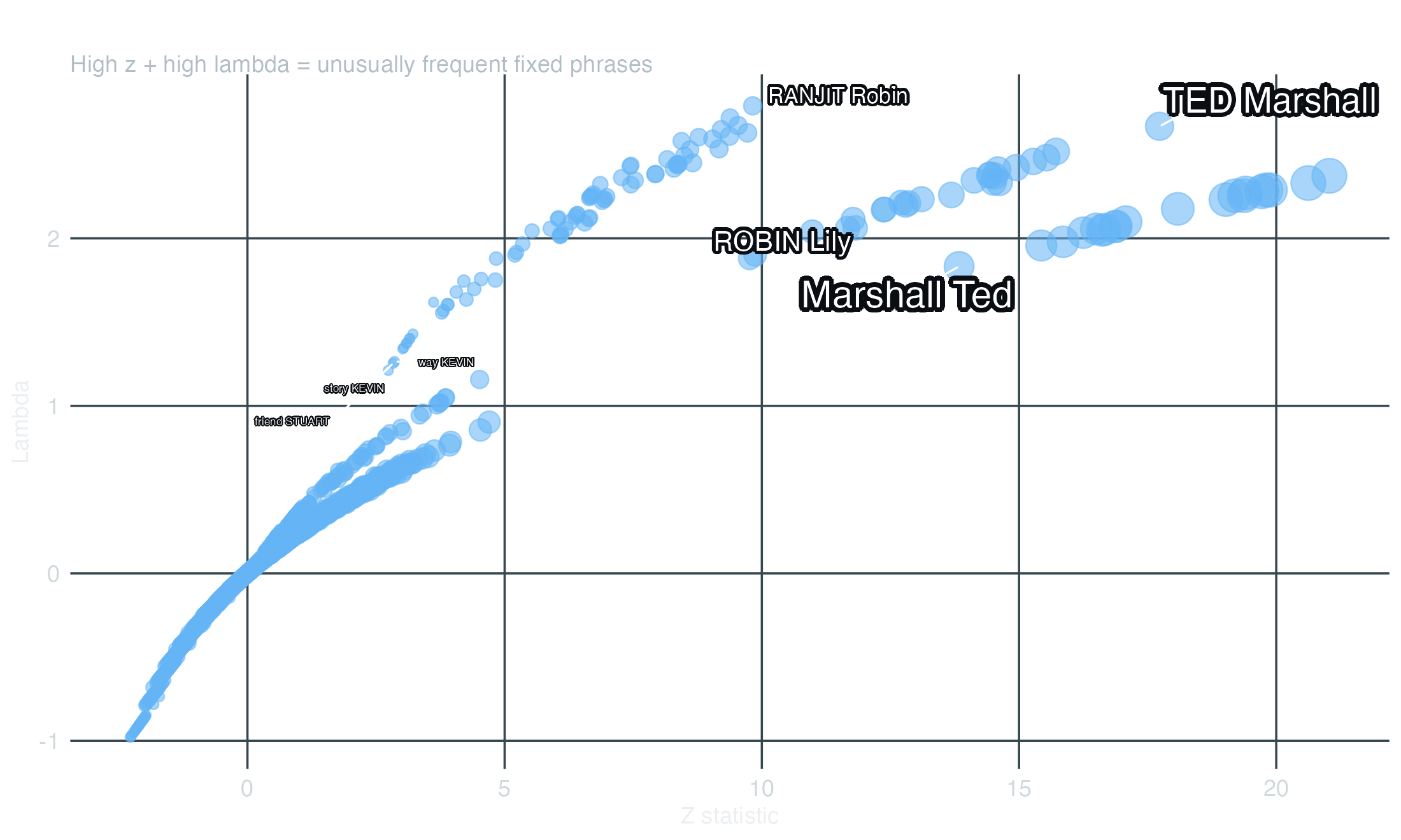
toks_s1 <- corp_himym |>
  corpus_subset(scripts$season == 1) |>
  tokens(padding = TRUE) |>
  tokens_remove(stopwords("english"))

colls_s1 <- textstat_collocations(toks_s1, tolower = FALSE, min_count = 5)

colls_s1 |>
  as_tibble() |>
  arrange(desc(z)) |>
  head(15)
#> # A tibble: 15 x 6
#>    collocation     count count_nested length lambda     z
#>    <chr>           <int>        <int>  <dbl>  <dbl> <dbl>
#>  1 right now          35            0      2   5.92  20.4
#>  2 getting married    19            0      2   5.44  16.7
#>  3 party number       18            0      2   5.50  16.4
#>  4 number three       15            0      2   6.06  15.7
#>  5 get married        26            0      2   4.33  15.5
#>  6 best friend        12            0      2   5.82  14.3
#>  7 met Ted            13            0      2   4.96  13.5
#>  8 MUSIC PLAYING      17            0      2   9.26  13.4
#>  9 two months         12            0      2   4.92  13.4
#> 10 years ago           9            0      2   6.25  13.2
#> 11 rain dance          9            0      2   7.41  12.6
#> 12 last night         13            0      2   4.44  12.6
#> 13 Uncle Marshall     10            0      2   6.58  12.5
#> 14 high school        11            0      2   8.51  12.4
#> 15 check plus          7            0      2   7.80  12.0

The lambda column is the log-ratio of observed-to-expected co-occurrence; z is the standardised score. Plotting them surfaces the phrases that are both frequent and unusually so:

collocations-plot.R

colls_df <- as_tibble(colls_s1) |>
  # Strip non-ASCII glyphs from collocation labels — emoji, smart-quotes, em-
  # dashes etc. fall through to placeholder boxes ("U+2024") in the rendered
  # PNG because ragg's bundled fonts do not carry those code points.
  mutate(collocation = gsub("[^\\x20-\\x7E]", "", collocation, perl = TRUE)) |>
  filter(nchar(collocation) > 0)

ggplot(colls_df, aes(x = z, y = lambda)) +
  geom_point(aes(size = count), color = "#64B5F6", alpha = 0.55) +
  geom_text_repel(
    data = colls_df |> filter(z > 12),
    aes(label = collocation, size = count),
    color        = "#ffffff",
    bg.color     = "#0a0d12",
    bg.r         = 0.18,
    max.overlaps = 18,
    box.padding  = 0.45,
    seed         = 7
  ) +
  scale_size_continuous(range = c(2, 8), guide = "none") +
  labs(x = "Z statistic", y = "Lambda",
       title = "HIMYM Season 1 — multi-word collocations",
       subtitle = "High z + high lambda = unusually frequent fixed phrases") +
  theme_dark_transparent()

The network, in motion

Scroll to see how co-occurrence builds from tokens to edges.

At each token position, the FCM counts every other character that appears within the window. The gold tokens fall inside the window — each pair increments a cell in the matrix.

Repeat that count across 208 episodes, every token position, every character pair: the result is a matrix of co-occurrence counts. A high cell value means those two characters appear in dialogue near each other often.

textplot_network() converts the FCM into a graph. Edge thickness scales with the cell value. The five principals cluster at the centre; edge weight makes the strongest relationships visible without looking at the matrix.

  Appendix — spaCy / spaCyr (POS tagging)

The original workshop also ran spaCyr — an R wrapper around the Python spaCy package — to tag every token as a noun, verb, adjective, or proper noun, then built an adjective wordcloud and an adjective frequency line plot per season. That section is not re-executed here because spaCyr requires a Python environment plus the en_core_web_sm model — a heavy dependency to ask of every site build.

spacy-demo.R

library(spacyr)
spacy_install()
spacy_initialize(model = "en_core_web_sm")

# Parse the whole corpus — pos column gets the part-of-speech tag
parsed <- spacy_parse(scripts, tag = TRUE)

# Keep adjectives only, then drop noise
adjectives <- parsed |> filter(pos == "ADJ") |> pull(lemma) |> unique()

toks_adj <- corp_himym |>
  tokens(remove_punct = TRUE, remove_numbers = TRUE, remove_symbols = TRUE) |>
  tokens_keep(adjectives) |>
  tokens_remove(c(stopwords("english"), "oh", "yeah", "okay", "like",
                  "get", "got", "can", "one", "hey", "go", "just",
                  "know", "well", "right", "even", "see"))

# Comparison wordcloud across seasons (max 8 groups)
dfm_adj <- toks_adj |>
  tokens_group(groups = paste("Season", scripts$season)) |>
  dfm() |>
  dfm_subset(scripts$season < 9)

textplot_wordcloud(dfm_adj, comparison = TRUE, rotation = 0.25,
                   min_size = 1, max_size = 5,
                   color = ggsci::pal_lancet()(8))

The full rendered version (with the comparison wordcloud and the per-season adjective frequency line plot) is in the original notebook on GitHub Pages.

  Where to go next

You now have most of the workshop pipeline: corpus → tokens → DFM → frequency, KWIC, similarity/distance dendrograms, character-frequency tracking, principal/secondary wordclouds, character-network graphs, and multi-word collocations. From here the package extends in several directions:

• textstat_keyness — features that distinguish one group of documents from another (e.g., what’s distinctive about Season 9 versus the rest)
• textstat_simil / textstat_dist — episode-to-episode similarity / distance, scaled to the full corpus
• quanteda.textmodels — supervised classifiers (Naive Bayes, SVM) and scaling models (Wordfish, Wordscores)
• textstat_collocations — multi-word expressions that occur together more than chance
• spaCyr — POS tagging and named-entity recognition (see appendix above)

The official site at quanteda.io has the canonical reference, and the workshop’s full case study is in the source repository.

  Workshop presentation

IDS Workshop slides — Hertie School, Fall 2022 Open fullscreen

Use the arrows or click on slides to navigate. Open fullscreen for keyboard control.

  Citation

Roa, J., Fonseca, A., & Kraess, A. (2022). How We Met Quanteda — Text Analysis with R. I2DS Tools for Data Science Workshop, M.Sc. Data Science for Public Policy, Hertie School, Berlin.

  Original notebook (full case study)     View the presentation     Source on GitHub